First Order and Second Order Continuous Temporal Systems

First Order

Time Domain

$$\tau \frac{\mathrm{d}y(t)}{\mathrm{d}t}+y(t)=x(t)$$

then

$$H(j\omega )=\frac{1}{j\omega \tau +1}$$

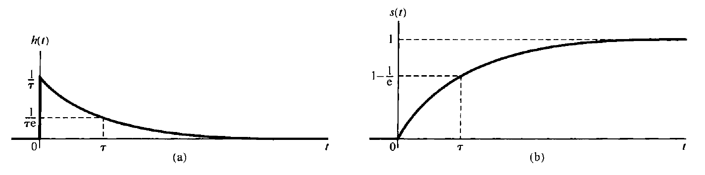
⇒ impulse response

$$h(t)=\frac{1}{\tau }\exp \left(-\frac{t}{\tau }\right)u(t)$$

⇒ step response

$$s(t)=h(t)\ast u(t)=\left[1-\exp \left(-\frac{t}{\tau }\right)\right]u(t)$$

where $\tau$ is the time constant of the system. (see the figure below)

Frequency Domain

Draw the Bode Plot of the system 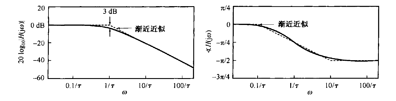The logarithmic modulus characteristic of a first-order system is an asymptotic straight line in both the low-frequency and high-frequency domains. And in low-frequency $\omega <\frac{1}{\tau }$, we have near zero magnitude response from the system.

We call $\omega =\frac{1}{\tau }$ the break frequency, where we have

$$20{\log }_{10}\left|H\left(j\frac{1}{\tau }\right)\right|\approx -3\mathrm{dB}$$

So we can also call it the 3dB point.

Second Order

Time Domain

$$\frac{{\mathrm{d}}^{2}y(t)}{\mathrm{d}{t}^2}+2\zeta {\omega }_n\frac{\mathrm{d}y(t)}{\mathrm{d}t}+{\omega }_n^{2}y(t)={\omega }_n^{2}x(t)$$

⇒

$$H(j\omega )=\frac{{\omega }_n^2}{(j\omega {)}^2+2\zeta {\omega }_n(j\omega )+{\omega }_n^2}=\frac{{\omega }_n^2}{(j\omega -c_1)(j\omega -c_2)}$$

where

$$\begin{array}{rl}{c}_1& =-\zeta {\omega }_n+{\omega }_n\sqrt{{\zeta }^2-1}\\ c_2& =-\zeta {\omega }_n-{\omega }_n\sqrt{{\zeta }^2-1}\end{array}$$

⇒

$$h(t)=\frac{{\omega }_n\exp \left(-\zeta {\omega }_{n}t\right)}{\sqrt{1-{\zeta }^2}}\left[\sin \left({\omega }_n\sqrt{1-{\zeta }^2}\right)t\right]u(t)$$

We call

• $\zeta$: damping ratio
• ${\omega }_n$: undamped natural frequency

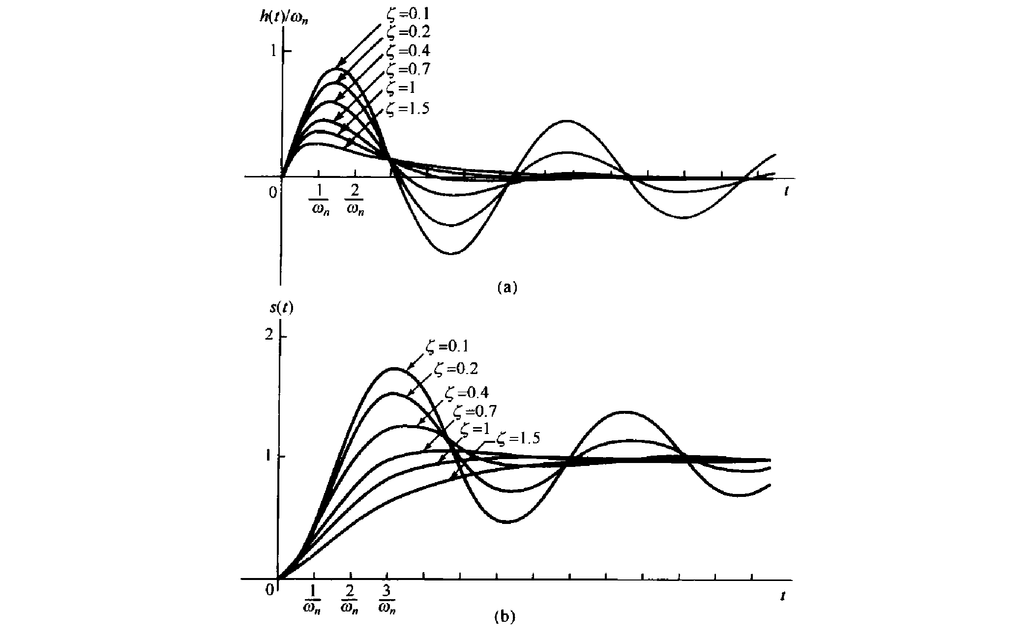
Note: the oscillating frequency ${\omega }_n\sqrt{1-{\zeta }^2}$ is always less than ${\omega }_n$ unless there is no damp (i.e. $\zeta =0$). That's why ${\omega }_n$ is called the undamped natural frequency.

Cases

• $\zeta <1$: Underdamped. Having overshoot and oscillation
• $\zeta =1$: Critically Damped. Fast and no overshoot
• $\zeta >1$: Overdamped. No overshoot but more slow to converge

Frequency Domain

Bode Plot: 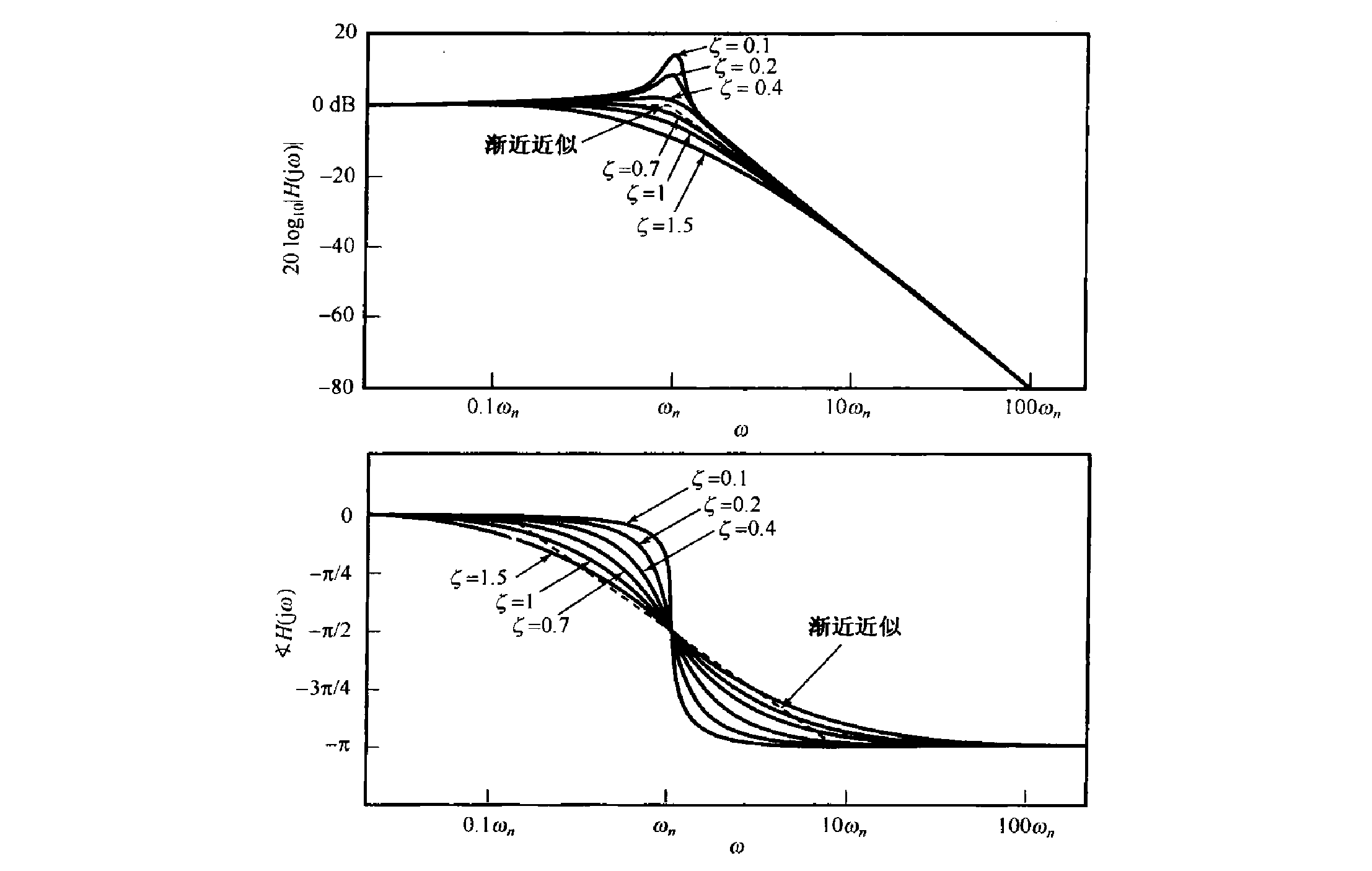We can still detect a breaking point at $\omega ={\omega }_n$. At both sides of the breaking point we can have a asymptotic straight line.

$\left|H(j\omega )\right|$ reaches it highest point at

$$\left({\omega }_n\sqrt{1-2{\zeta }^2},\frac{1}{2\zeta \sqrt{1-{\zeta }^2}}\right)$$

when $\zeta <\frac{\sqrt{2}}{2}$.

The fact that $H(j\omega )$ may have a peak value is very important in designing frequency-selective filters and selective amplifiers. In some applications, it may be desirable to design such circuits so that their magnitude response has a sharp peak at a given frequency, thereby providing selectivity within a relatively narrow range of frequencies.

This type of circuit uses the quality factor ($Q$) to measure the sharpness of the peak. For a second-order circuit, Q is usually taken as:

$$Q=\frac{1}{2\zeta }$$

That is, less dampness leads to more sharpness