Support Vector Machine - SVM

Classifier

For parameters $w,b$, write our classifier as

$$h_{w,b}(x)=g(w^{T}x+b)$$

Here, $g(z)=1$ if $z\ge 0$, and $g(z)=-1$ otherwise.

Note

A bigger $\left|{\omega }^{T}x+b\right|$ indicates a more confident prediction.

Functional Margin

Given a training example $(x^{(i)},y^{(i)})$, we define the functional margin of $(w,b)$ as

$${\hat{\gamma }}^{(i)}=y^{(i)}\left({\omega }^T{x}^{(i)}+b\right)$$

Note that if $y^{(i)}=1$, then for the functional margin to be large (i.e., for our prediction to be confident and correct), we need $w^T{x}^{(i)}+b$ to be a large positive number. Conversely, if $y^{(i)}=-1$, then for the functional margin to be large, we need $w^T{x}^{(i)}+b$ to be a large negative number. Moreover, if $y^{(i)}(w^T{x}^{(i)}+b)>0$, then our prediction on this example is correct. Hence, a large functional margin represents a confident and a correct prediction.

Given a training set $S=\left\{(x^{(i)},y^{(i)})\mid i=1,2,\dots ,n\right\}$, we also define the function margin of $(w,b)$ with respect to $S$ as the smallest of the functional margins of the individual training examples. Denoted by $\hat{\gamma }$, this can therefore be written:

$$\hat{\gamma }=\underset{i=1,\dots ,n}{\min }{\hat{\gamma }}^{(i)}$$

Issues with this form

For a linear classifier with the choice of $g$ given above (taking values in $\{-1,1\}$), there's one property of the functional margin that makes it not a very good measure of confidence. Given our choice of $g$, we note that if we replace $w$ with $2w$ and $b$ with $2b$, then since $g(w^{T}x+b)=g(2w^{T}x+2b)$, this would not change $h_{w,b}(x)$ at all. However, replacing $(w,b)$ with $(2w,2b)$ also results in multiplying our functional margin by a factor of $2$. Thus, it seems that by exploiting our freedom to scale $w$ and $b$, we can make the functional margin arbitrarily large without really changing anything meaningful. Intuitively, it might therefore make sense to impose some sort of normalization condition such as that $\Vert w{\Vert }_2=1$; i.e., we might replace $(w,b)$ with $(w/\Vert w{\Vert }_2,b/\Vert w{\Vert }_2)$, and instead consider the functional margin of $(w/\Vert w{\Vert }_2,b/\Vert w{\Vert }_2)$.

Geometric Margin

Consider the picture below

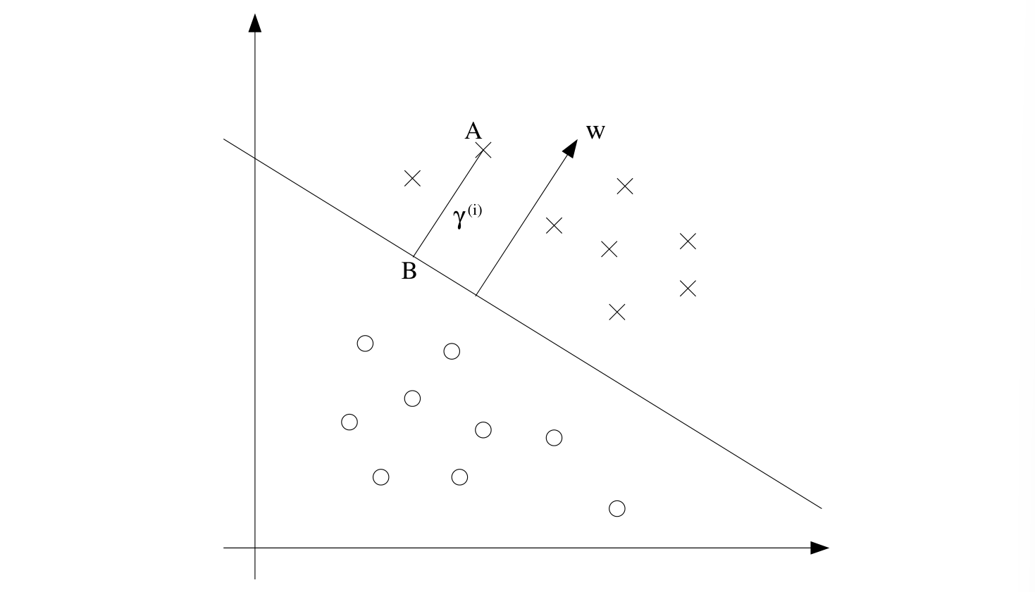
The decision boundary corresponding to $(w,b)$ is shown, along with the vector $w$. Note that $w$ is orthogonal (at 90°) to the separating hyperplane. Consider the point at A, which represents the input $x^{(i)}$ of some training example with label $y^{(i)}=1$. Its distance to the decision boundary, ${\gamma }^{(i)}$, is given by the line segment AB.

Since $B$ is on the decision boundary $w^{T}x+b=0$, we have

$$w^T\left(x^{(i)}-{\gamma }^{(i)}\frac{w}{\Vert w\Vert }\right)+b=0$$

Solving for ${\gamma }^{(i)}$ yields

$${\gamma }^{(i)}={\left(\frac{w}{\Vert w\Vert }\right)}^T{x}^{(i)}+\frac{b}{\Vert w\Vert }$$

More generally, we define the geometric margin of $(w,b)$ with respect to a training example $(x^{(i)},y^{(i)})$ to be

$${\gamma }^{(i)}=y^{(i)}\left[{\left(\frac{w}{\Vert w\Vert }\right)}^T{x}^{(i)}+\frac{b}{\Vert w\Vert }\right]$$

Note that if $\Vert w\Vert =1$, then the functional margin equals the geometric margin.

The Optimal Margin Classifier

Note

For now, we will assume that we are given a training set that is linearly separable.

Form 1

To maximize the geometric margin, we could pose the following optimization problem

$$\begin{array}{rl}\underset{\gamma ,w,b}{\max }& \gamma \\ \text{s.t.}& y^{(i)}\left(w^T{x}^{(i)}+b\right)\ge \gamma ,i=1,2,\dots ,n\\ & \Vert w\Vert =1\end{array}$$

If we could solve the optimization problem above, we'd be done. But the "$\Vert w\Vert =1$" constraint is a nasty (non-convex) one, and this problem certainly isn't in any format that we can plug into standard optimization software to solve.

Form 2

So, let's try transforming the problem into a nicer one. Consider:

$$\begin{array}{rl}\underset{\hat{\gamma },w,b}{\max }& \frac{\hat{\gamma }}{\Vert w\Vert }\\ \text{s.t.}& y^{(i)}\left(w^T{x}^{(i)}+b\right)\ge \hat{\gamma },i=1,2,\dots ,n\end{array}$$

Here, we're going to maximize $\hat{\gamma }/\Vert w\Vert$, subject to the functional margins all being at least $\hat{\gamma }$. Since the geometric and functional margins are related by $\gamma =\hat{\gamma }/\Vert w\Vert$, this will give us the answer we want. Moreover, we've gotten rid of the constraint $\Vert w\Vert =1$ that we didn't like. The downside is that we now have a nasty (again, non-convex) objective $\frac{\hat{\gamma }}{\Vert w\Vert }$ function.

Form 3

Recall our earlier discussion that we can add an arbitrary scaling constraint on $w$ and $b$ without changing anything. Therefore, we introduce the scaling constraint that the functional margin of $w,b$ with respect to the training set must be $1$:

$$\hat{\gamma }=1$$

This restriction can be satisfied by rescaling $w,b$. Noting that maximizing $\hat{\gamma }/\Vert w\Vert =1/\Vert \omega \Vert$ is the same thing minimizing $\Vert w{\Vert }^2$, we now have the following optimization problem:

$$\begin{array}{rl}\underset{w,b}{\min }& \frac{1}{2}{\Vert w\Vert }^2\\ \text{s.t.}& y^{(i)}\left(w^T{x}^{(i)}+b\right)\ge 1,i=1,2,\dots ,n\end{array}$$

We've now transformed the problem into a form that can be efficiently solved.

Lagrange Duality

Primal Problem

Consider the following, which we'll call the primal optimization problem:

$$\begin{array}{rl}\underset{w}{\min }& f(w)\\ \text{s.t.}& g_i(w)\le 0,i=1,\dots ,k\\ & h_i(w)=0,i=1,\dots ,l\end{array}$$

To solve it, we start by defining the generalized Lagrangian

$$\mathcal{L}(w,\alpha ,\beta )=f(w)+\sum _{i=1}^k{\alpha }_i{g}_i(w)+\sum _{i=1}^l{\beta }_i{h}_i(w)$$

Here, the ${\alpha }_i$'s and ${\beta }_i$'s are the Lagrange multipliers. Consider the quantity

$${\theta }_{\mathcal{P}}(w)=\underset{\alpha ,\beta :\alpha \ge 0}{\max }\mathcal{L}(w,\alpha ,\beta ).$$

Here, the "$\mathcal{P}$" subscript stands for "primal." Let some $w$ be given. If $w$ violates any of the primal constraints (i.e., if either $g_i(w)>0$ or $h_i(w)\ne 0$ for some $i$), then you should be able to verify that

$$\begin{array}{rl}{\theta }_{\mathcal{P}}(w)& =\underset{\alpha ,\beta :{\alpha }_i\ge 0}{\max }f(w)+\sum _{i=1}^k{\alpha }_i{g}_i(w)+\sum _{i=1}^l{\beta }_i{h}_i(w)\\ & =\infty \end{array}$$

Conversely, if the constraints are indeed satisfied for a particular value of $w$, then ${\theta }_{\mathcal{P}}(w)=f(w)$. Hence,

$${\theta }_{\mathcal{P}}(w)=\{\begin{array}{ll}f(w)& \text{if }w\text{ satisfies primal constraints.}\\ \infty & \text{otherwise.}\end{array}$$

Thus, ${\theta }_{\mathcal{P}}$ takes the same value as the objective in our problem for all values of w that satisfies the primal constraints, and is positive infinity if the constraints are violated. Hence, if we consider the minimization problem

$$\underset{w}{\min }{\theta }_{\mathcal{P}}(w)=\underset{w}{\min }\underset{\alpha ,\beta :{\alpha }_i\ge 0}{\max }\mathcal{L}(w,\alpha ,\beta ),$$

we see that it is the same problem (i.e., and has the same solutions as) our original, primal problem. For later use, we also define the optimal value of the objective to be $p^{\ast }={\min }_w{\theta }_{\mathcal{P}}(w)$; we call this the value of the primal problem.

Dual Problem

Now, let's look at a slightly different problem. We define

$${\theta }_{\mathcal{D}}(\alpha ,\beta )=\underset{w}{\min }\mathcal{L}(w,\alpha ,\beta ).$$

Here, the "$\mathcal{D}$" subscript stands for "dual." Note also that whereas in the definition of ${\theta }_{\mathcal{P}}$ we were optimizing (maximizing) with respect to $\alpha ,\beta$, here we are minimizing with respect to $w$.

We can now pose the dual optimization problem:

$$\underset{\alpha ,\beta :{\alpha }_i\ge 0}{\max }{\theta }_{\mathcal{D}}(\alpha ,\beta )=\underset{\alpha ,\beta :{\alpha }_i\ge 0}{\max }\underset{w}{\min }\mathcal{L}(w,\alpha ,\beta ).$$

This is exactly the same as our primal problem shown above, except that the order of the "max" and the "min" are now exchanged. We also define the optimal value of the dual problem's objective to be $d^{\ast }={\max }_{\alpha ,\beta :{\alpha }_i\ge 0}{\theta }_{\mathcal{D}}(w)$.

How are the primal and the dual problems related? It can easily be shown that $d^{\ast }={\max }_{\alpha ,\beta :{\alpha }_i\ge 0}{\min }_w\mathcal{L}(w,\alpha ,\beta )\le {\min }_w{\max }_{\alpha ,\beta :{\alpha }_i\ge 0}\mathcal{L}(w,\alpha ,\beta )=p^{\ast }.$ this follows from the "max min" of a function always being less than or equal to the "min max." However, under certain conditions, we will have

$$d^{\ast }=p^{\ast },$$

so that we can solve the dual problem in lieu of the primal problem.

Karush-Kuhn-Tucker (KKT) conditions

Assumptions Suppose $f$ and the $g_i$'s are convex, and the $h_i$'s are affine (i.e. there exists $a_i,b_i$ so that $h_i(w)=a_i^{T}w+b_i$). Suppose further that constraints $g_i$ are (strictly) feasible (i.e. there exists some $w$ so that $g_i(w)<0$ for all $i$).

Claim There must exist $w^{\ast },{\alpha }^{\ast },{\beta }^{\ast }$ so that $w^{\ast }$ is the solution to the primal problem, ${\alpha }^{\ast },{\beta }^{\ast }$ are the solution to the dual problem, and moreover $p^{\ast }=d^{\ast }=\mathcal{L}(w^{\ast },{\alpha }^{\ast },{\beta }^{\ast })$.

and $w^{\ast },{\alpha }^{\ast },{\beta }^{\ast }$ satisfy the Karush-Kuhn-Tucker (KKT) conditions:

$$\begin{array}{rl}\frac{\partial }{\partial w_i}\mathcal{L}(w^{\ast },{\alpha }^{\ast },{\beta }^{\ast })& =0,i=1,\dots ,d\\ \frac{\partial }{\partial {\beta }_i}\mathcal{L}(w^{\ast },{\alpha }^{\ast },{\beta }^{\ast })& =0,i=1,\dots ,l\\ {\alpha }_i^{\ast }{g}_i(w^{\ast })& =0,i=1,\dots ,k\\ g_i(w^{\ast })& \le 0,i=1,\dots ,k\\ {\alpha }^{\ast }& \ge 0,i=1,\dots ,k\end{array}$$

The Dual Form of SVM

Support Vectors

Previously, we posed the following (primal) optimization problem for finding the optimal margin classifier

$$\begin{array}{rl}\underset{w,b}{\min }& \frac{1}{2}{\Vert w\Vert }^2\\ \text{s.t.}& y^{(i)}\left(w^T{x}^{(i)}+b\right)\ge 1,i=1,2,\dots ,n\end{array}$$

We can write the constraints as

$$g_i(w)=-y^{(i)}(w^T{x}^{(i)}+b)+1\le 0$$

We have one such constraint for each training example. Note that from the KKT dual complementarity condition, we will have ${\alpha }_i>0$ only for the training examples that have functional margin exactly equal to one (i.e., the ones corresponding to constraints that hold with equality, $g_i(w)=0$). Consider the figure below, in which a maximum margin separating hyperplane is shown by the solid line. The points with the smallest margins are exactly the ones closest to the decision boundary; here, these are the three points (one negative and two positive examples) that lie on the dashed lines parallel to the decision boundary. Thus, only three of the ${\alpha }_i$’s—namely, the ones corresponding to these three training examples—will be non-zero at the optimal solution to our optimization problem. These three points are called the support vectors in this problem.

Find the dual problem

Now we construct the Lagrangian for SVM, we have

$$\mathcal{L}(w,b,\alpha )=\frac{1}{2}\Vert w{\Vert }^2-\sum _{i=1}^n{\alpha }_i\left[y^{(i)}(w^T{x}^{(i)}+b)-1\right]$$

Note that there're only "${\alpha }_i$" but no "${\beta }_i$" Lagrange multipliers, since the problem has only inequality constraints. To find the dual form of the problem, we need to first minimize $\mathcal{L}(w,b,\alpha )$ with respect to $w$ and $b$ (for fixed $\alpha$), to get ${\theta }_{\mathcal{D}}$, via setting the derivatives of $\mathcal{L}$ with respect to $w$ and $b$ to zero

$$\{\begin{array}{l}{\nabla }_w\mathcal{L}(w,b,\alpha )=w-\sum _{i=1}^n{\alpha }_i{y}^{(i)}{x}^{(i)}=0⟹w=\sum _{i=1}^n{\alpha }_i{y}^{(i)}{x}^{(i)}\\ \frac{\partial }{\partial b}\mathcal{L}(w,b,\alpha )=\sum _{i=1}^n{\alpha }_i{y}^{(i)}=0.\end{array}$$

Taking these results into the original Lagrangian

$$\Vert w{\Vert }^2=w^{T}w={\left(\sum _{i=1}^n{\alpha }_i{y}^{(i)}{x}^{(i)}\right)}^T\left(\sum _{j=1}^n{\alpha }_j{y}^{(j)}{x}^{(j)}\right)=\sum _{i,j=1}^n{\alpha }_i{\alpha }_j{y}^{(i)}{y}^{(j)}(x^{(i)}{)}^T{x}^{(j)}$$

and

$$\begin{array}{rl}\sum _{i=1}^n{\alpha }_i{y}^{(i)}(w^T{x}^{(i)}+b)& =\sum _{i=1}^n{\alpha }_i{y}^{(i)}\left({\left(\sum _{j=1}^n{\alpha }_j{y}^{(j)}{x}^{(j)}\right)}^T{x}^{(i)}+b\right)\\ & =\sum _{i=1}^n{\alpha }_i{y}^{(i)}\left(\sum _{j=1}^n{\alpha }_j{y}^{(j)}(x^{(j)}{)}^T{x}^{(i)}+b\right)\\ & =\sum _{i,j=1}^n{\alpha }_i{\alpha }_j{y}^{(i)}{y}^{(j)}(x^{(i)}{)}^T{x}^{(j)}+b\sum _{i=1}^n{\alpha }_i{y}^{(i)}\end{array}$$

With ${\sum }_{i=1}^n{\alpha }_i{y}^{(i)}=0$, we get the final result

$$\mathcal{L}(w,b,\alpha )=\sum _{i=1}^n{\alpha }_i-\frac{1}{2}\sum _{i,j=1}^n{\alpha }_i{\alpha }_j{y}^{(i)}{y}^{(j)}(x^{(i)}{)}^T{x}^{(j)}$$

Putting this together with the constraints ${\alpha }_i\ge 0$ (that we always had) and the constraint of ${\alpha }_i{y}^i$, we obtain the following dual optimization problem

$$\begin{array}{rl}\underset{\alpha }{\max }& \mathcal{L}(\alpha )=\sum _{i=1}^n{\alpha }_i-\frac{1}{2}\sum _{i,j=1}^n{\alpha }_i{\alpha }_j{y}^{(i)}{y}^{(j)}(x^{(i)}{)}^T{x}^{(j)}\\ \text{s.t.}& {\alpha }_i\ge 0,i=1,2,\dots ,n\\ & \sum _{i=1}^n{\alpha }_i{y}^{(i)}=0\end{array}$$

Regularization and the Non-separable Case

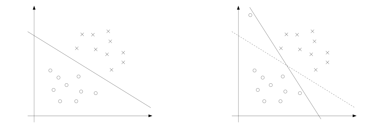
The derivation of the SVM as presented so far assumed that the data is linearly separable. While mapping data to a high dimensional feature space via $\varphi$ does generally increase the likelihood that the data is separable, we can't guarantee that it always will be so. Also, in some cases it is not clear that finding a separating hyperplane is exactly what we'd want to do, since that might be susceptible to outliers. For instance, the left figure below shows an optimal margin classifier, and when a single outlier is added in the upper-left region (right figure), it causes the decision boundary to make a dramatic swing, and the resulting classifier has a much smaller margin.

To make the algorithm work for non-linearly separable datasets as well as be less sensitive to outliers, we reformulate our optimization (using ${\ell }_1$ regularization) as follows:

$$\begin{array}{rl}\underset{\xi ,w,b}{\min }& \frac{1}{2}{\Vert w\Vert }^2+C\sum _{i=1}^n{\xi }_i\\ \text{s.t.}& y^{(i)}\left(w^T{x}^{(i)}+b\right)\ge 1-{\xi }_i,i=1,2,\dots ,n\\ & {\xi }_i\ge 0,i=1,2,\dots ,n\end{array}$$

Thus, examples are now permitted to have (functional) margin less than $1$, and if an example has functional margin $1-{\xi }_i$ (with ${\xi }_i>0$), we would pay a cost of the objective function being increased by $C{\xi }_i$ . The parameter $C$ controls the relative weighting between the twin goals of making the $\Vert w{\Vert }^2$ small (which we saw earlier makes the margin large) and of ensuring that most examples have functional margin at least $1$.