Linear Models

Discriminant Function

Binary Classification

$$g(\mathbf{x})={\mathbf{w}}^T\mathbf{x}+w_0$$

Criteria:

$$\mathbf{x}\in {\omega }_1⟺g(\mathbf{x})>0;\mathbf{x}\in {\omega }_2⟺g(\mathbf{x})<0$$

Here ${\mathbf{w}}^T\mathbf{x}+\mathbf{w}=0$ is the separating surface

Loss Function

Classification

$$L(f,D)=\frac{1}{N}\sum _{i=1}^{n}l\left(f(x_i)\ne y_i\right)$$

Regression

$$L(f,D)=\frac{1}{N}\sum _{i=1}^n{\left(f(x_i)-y_i\right)}^2$$

Least Squares Method

For linear function $f(\mathbf{x})={\mathbf{w}}^T\mathbf{x}={\mathbf{x}}^T\mathbf{w}$, where

$$\mathbf{w}=[w_0,w_1,\dots ,w_d{]}^T,\mathbf{x}={\left[1,x_1,\dots ,x_d\right]}^T$$

$\mathbf{x}$ is the augmented sample vector.

For $n$ samples ${\mathbf{x}}^{(1)},\dots ,{\mathbf{x}}^{(n)}$, we define the design matrix

$$\mathbf{X}=\left(\begin{array}{c}-{\left({\mathbf{x}}^{(1)}\right)}^T-\\ -{\left({\mathbf{x}}^{(2)}\right)}^T-\\ ⋮\\ -{\left({\mathbf{x}}^{(n)}\right)}^T-\end{array}\right)$$

and

$$\mathbf{y}=\left(\begin{array}{c}{y}^{(1)}\\ y^{(2)}\\ ⋮\\ y^{(n)}\end{array}\right)$$

we have

$$\mathbf{X}\mathbf{w}-\mathbf{y}=\left(\begin{array}{c}f({\mathbf{x}}^{(1)})-y^{(1)}\\ f({\mathbf{x}}^{(2)})-y^{(2)}\\ ⋮\\ f({\mathbf{x}}^{(n)})-y^{(n)}\end{array}\right)$$

we want to minimize

$$E(\mathbf{w})=\frac{1}{N}\sum _{j=1}^N{\left(f({\mathbf{x}}^{(j)})-y^{(j)}\right)}^2=\frac{1}{N}(\mathbf{X}\mathbf{w}-\mathbf{y}{)}^T(\mathbf{X}\mathbf{w}-\mathbf{y})$$

the solution is

$${\mathbf{w}}^{\ast }={\left({\mathbf{X}}^T\mathbf{X}\right)}^{-1}{\mathbf{X}}^T\mathbf{y}$$

Linear Discriminant Analysis

When working with high-dimensional datasets it is important to apply dimensionality reduction techniques to make data exploration and modeling more efficient. One such technique is Linear Discriminant Analysis (LDA) which helps in reducing the dimensionality of data while retaining the most significant features for classification tasks. It works by finding the linear combinations of features that best separate the classes in the dataset.

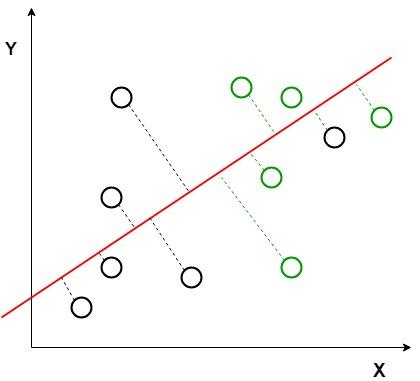Image shows an example where the classes (black and green circles) are not linearly separable. LDA attempts to separate them using red dashed line. It uses both axes (X and Y) to generate a new axis in such a way that it maximizes the distance between the means of the two classes while minimizing the variation within each class. This transforms the dataset into a space where the classes are better separated.

Logistic Regression

We could approach the classification problem ignoring the fact that $y$ is discrete-valued, and use our old linear regression algorithm to try to predict $y$ given $x$. However, it is easy to construct examples where this method performs very poorly. Intuitively, it also doesn't make sense for $h_{\theta }(x)$ to take values larger than $1$ or smaller than $0$ when we know that $y\in \{0,1\}$. To fix this, let's change the form for our hypotheses $h_{\theta }(x)$. We will choose

$$h_{\theta }(x)=g({\theta }^{T}x)=\frac{1}{1+e^{-{\theta }^{T}x}},$$

where

$$g(z)=\frac{1}{1+e^{-z}}$$

is called the logistic function or the sigmoid function.

Let us assume that

$$\begin{array}{rl}P(y=1\mid x;\theta )& =h_{\theta }(x)\\ P(y=0\mid x;\theta )& =1-h_{\theta }(x)\end{array}$$

Note that this can be written more compactly as

$$p(y\mid x;\theta )=(h_{\theta }(x){)}^y(1-h_{\theta }(x){)}^{1-y}$$

Assuming that the $n$ training examples were generated independently, we can then write down the likelihood of the parameters as

$$\begin{array}{rl}L(\theta )& =p(\vec{y}\mid X;\theta )\\ & =\prod _{i=1}^{n}p(y^{(i)}\mid x^{(i)};\theta )\\ & =\prod _{i=1}^n(h_{\theta }(x^{(i)}){)}^{y^{(i)}}(1-h_{\theta }(x^{(i)}){)}^{1-y^{(i)}}\end{array}$$

As before, it will be easier to maximize the log likelihood:

$$\ell (\theta )=\log L(\theta )=\sum _{i=1}^n{y}^{(i)}\log h_{\theta }(x^{(i)})+(1-y^{(i)})\log (1-h_{\theta }(x^{(i)}))$$

Similar to our derivation in the case of linear regression, we can use gradient ascent. Written in vectorial notation, our updates will therefore be given by $\theta :=\theta +\alpha {\nabla }_{\theta }\ell (\theta )$. (Note the positive rather than negative sign in the update formula, since we're maximizing, rather than minimizing, a function now.) Let's start by working with just one training example $(x,y)$, and take derivatives to derive the stochastic gradient ascent rule:

$$\begin{array}{rl}\frac{\partial }{\partial {\theta }_j}\ell (\theta )& =\left(y\frac{1}{g({\theta }^{T}x)}-(1-y)\frac{1}{1-g({\theta }^{T}x)}\right)\frac{\partial }{\partial {\theta }_j}g({\theta }^{T}x)\\ & =\left(y\frac{1}{g({\theta }^{T}x)}-(1-y)\frac{1}{1-g({\theta }^{T}x)}\right)g({\theta }^{T}x)(1-g({\theta }^{T}x))\frac{\partial }{\partial {\theta }_j}{\theta }^{T}x\\ & =(y(1-g({\theta }^{T}x))-(1-y)g({\theta }^{T}x))x_j\\ & =(y-h_{\theta }(x))x_j\end{array}$$

This therefore gives us the stochastic gradient ascent rule

$${\theta }_j:={\theta }_j+\alpha \left(y^{(i)}-h_{\theta }\left(x^{(i)}\right)\right)x_j^{(i)}$$

Perceptron

Consider modifying the logistic regression method to force it to output values that are either $0$ or $1$ or exactly. To do so, it seems natural to change the definition of $g$ to be the threshold function

$$g(z)=\{\begin{array}{ll}1,& \text{if}z\ge 0\\ 0,& \text{if}z<0\end{array}$$

If we then let $h_{\theta }(x)=g({\theta }^{T}x)$ as before but using this modified definition of $g$, and if we use the update rule

$${\theta }_j:={\theta }_j+\alpha \left(y^{(i)}-h_{\theta }\left(x^{(i)}\right)\right)x_j^{(i)}$$

then we have the perceptron learning algorithm.

Multi-Class Classification

We introduce $k$ groups of parameters ${\theta }_1,\dots ,{\theta }_k$, each of them being a vector in ${\mathbb{R}}^d$. Intuitively, we would like to use ${\theta }_1^{T}x,\dots ,{\theta }_k^{T}x$ to represent the probabilities $P(y=1\mid x;\theta ),\dots ,P(y=k\mid x;\theta )$. However, there are two issues with such a direct approach. First, ${\theta }_j^{T}x$ is not necessarily with $[0,1]$. Second, the summation of ${\theta }_j^{T}x$'s is not necessarily $1$. Instead, we will define the softmax function

$$\mathrm{softmax}(t_1,\dots ,t_k)=\left(\begin{array}{c}\frac{\exp (t_1)}{{\sum }_{j=1}^k\exp (t_j)}\\ ⋮\\ \frac{\exp (t_k)}{{\sum }_{j=1}^k\exp (t_j)}\end{array}\right)$$

The inputs to the softmax function, the vector $t$ here, are often called logits. The output of the softmax function is always a probability vector whose entries are non-negative and sum up to $1$.

Let $(t_1,\dots ,t_k)=({\theta }_1^{T}x,\dots ,{\theta }_k^{T}x)$, we obtain the following probabilistic model

$$\left(\begin{array}{c}P(y=1\mid x;\theta )\\ ⋮\\ P(y=k\mid x;\theta )\end{array}\right)=\mathrm{softmax}(t_1,\dots ,t_k)$$

that is

$$P(y=i\mid x;\theta )=\frac{\exp (t_i)}{{\sum }_{j=1}^k\exp (t_j)}=\frac{\exp ({\theta }_i^{T}x)}{{\sum }_{j=1}^k\exp ({\theta }_j^{T}x)}$$

The negative log-likelihood of a single example $(x,y)$, $y\in \left\{1,2,\dots ,k\right\}$ is

$$-\log p(y\mid x,\theta )=-\log \left(\frac{\exp (t_y)}{{\sum }_{j=1}^k\exp (t_j)}\right)$$

Thus the loss function is given as

$$\ell (\theta )=\sum _{i=1}^n-\log \left(\frac{\exp \left({\theta }_{y^{(i)}}^T{x}^{(i)}\right)}{{\sum }_{j=1}^k\exp \left({\theta }_{y^{(i)}}^T{x}^{(i)}\right)}\right)$$

It's convenient to define the cross-entropy loss ${\ell }_{\mathrm{ce}}:{\mathbb{R}}^k\times \left\{1,2,\dots ,k\right\}\to {\mathbb{R}}_{\ge 0}$, which modularizes in the complex equation above

$${\ell }_{\mathrm{ce}}\left((t_1,\dots ,t_k),y\right)=-\log \left(\frac{\exp (t_y)}{{\sum }_{j=1}^k\exp (t_j)}\right)$$

With this notation, we can simply rewrite the total loss into

$$\ell (\theta )=\sum _{i=1}^n{\ell }_{\mathrm{ce}}\left(\left({\theta }_1^T{x}^{(i)},\dots ,{\theta }_k^T{x}^{(i)}\right),y^{(i)}\right)$$

Support Vector Machine

Support Vector Machine - SVM