Adversarial Search

Games

We first consider games with two players, whom we call MAX and MIN. MAX moves first, and then they take turns moving until the game is over. A can can be formally defined as a kind of search problem with the following elements:

• $S_0$: The initial state, which specifies how the game is set up at the start
• $\mathrm{PLAYER}(s)$: Defines which player has the move in a state.
• $\mathrm{ACTIONS}(\mathrm{s})$: Returns the set of legal moves in a state.
• $\mathrm{RESULT}(s,a)$: The transition model, which defines the result of a move
• $\mathrm{TERMINAL}-\mathrm{TEST}(s)$: A terminal test, which is true when the game is over and false otherwise. States where the game has ended are called terminal states
• $\mathrm{UTILITY}(s,p)$. A utility function, defines the final numeric value for a game that ends in terminal state $s$ for a player $p$. In chess, the outcome is a win, loss, or draw, which can value $+1$, $0$ and $\frac{1}{2}$. A zero-sum game is defined as one where the total payoff to all players is the same for every instance of the game. (So "constant-sum" would have been a better term).

The initial state, $\mathrm{ACTIONS}$ function, and $\mathrm{RESULT}$ function define the game tree for the game—a tree where the nodes are game states and the edges are moves.

Optimal Decisions in Games

Minimax decision

Given a game tree, the optimal strategy can be determined from the minimal value of each node, which we write a MINIMAX(n). The minimax value of a node is the utility (for MAX) of being in the corresponding state, assuming that both players play optimally from there to the end of the game. Obviously, the minimax value of a terminal state is just its utility. Furthermore, given a choice, MAX prefers to move to a state of maximum value, whereas MIN prefers a state of minimum value. So we have the following

$$\begin{array}{rl}& \mathrm{MINIMAX}(s)=\\ & \{\begin{array}{ll}\mathrm{UTILITY}(s),& \mathrm{TERMINAL}(s)\\ {\max }_{a\in \mathrm{ACTIONS}(s)}\mathrm{MINIMAX}(\mathrm{RESULT}(s,a)),& \mathrm{PLAYER}(s)=\mathrm{MAX}\\ {\min }_{a\in \mathrm{ACTIONS}(s)}\mathrm{MINIMAX}(\mathrm{RESULT}(s,a)),& \mathrm{PLAYER}(s)=\mathrm{MIN}\end{array}\end{array}$$

The minimax algorithm

import math
 
def minimax(current_state, depth, maximizing_player, get_possible_moves, evaluate_state):
    """
    Implements the minimax search algorithm.
 
    Args:
        current_state: The current state of the game.
        depth: The current depth in the search tree.
        maximizing_player: True if the current player is the maximizing player, False otherwise.
        get_possible_moves: A function that takes the current state and returns a list of possible next states.
        evaluate_state: A function that takes a state and returns its score.
                        Positive score is good for the maximizing player, negative for the minimizing player.
 
    Returns:
        The best score for the current player from this state.
    """
    if depth == 0 or is_terminal_state(current_state):  # Base case: reached max depth or terminal state
        return evaluate_state(current_state)
 
    if maximizing_player:
        max_eval = -math.inf
        for next_state in get_possible_moves(current_state):
            eval = minimax(next_state, depth - 1, False, get_possible_moves, evaluate_state)
            max_eval = max(max_eval, eval)
        return max_eval
    else:
        min_eval = math.inf
        for next_state in get_possible_moves(current_state):
            eval = minimax(next_state, depth - 1, True, get_possible_moves, evaluate_state)
            min_eval = min(min_eval, eval)
        return min_eval
 
def find_best_move(initial_state, depth, get_possible_moves, evaluate_state):
    """
    Finds the best move for the maximizing player from the initial state using minimax.
 
    Args:
        initial_state: The starting state of the game.
        depth: The maximum depth to search.
        get_possible_moves: A function that takes the current state and returns a list of possible next states.
        evaluate_state: A function that takes a state and returns its score.
 
    Returns:
        The best next state for the maximizing player.
    """
    best_move = None
    max_eval = -math.inf
 
    for next_state in get_possible_moves(initial_state):
        eval = minimax(next_state, depth - 1, False, get_possible_moves, evaluate_state)
        if eval > max_eval:
            max_eval = eval
            best_move = next_state
    return best_move
 

The minimax algorithm performs a complete depth-first exploration of the game tree. If the maximum depth of the tree is $m$ and there are $b$ legal moves at each point, then the time complexity of the minimax algorithm is $O(b^m)$.

Optimal decisions in multiplayer games

Instead of returning a single score representing the outcome for one player, the minimax function in a multiplayer setting typically returns a tuple (or a vector) of scores, where each element in the tuple corresponds to the score of a specific player.

Recursive Step:

• Determine whose turn it is in the current state. Let's say it's player $p$ 's turn.
• Generate all possible next states that can be reached from the current state through player $p$ 's actions.
• For each next state, recursively call the Minimax function to get the score tuple for that state.
• Player $p$ will choose the action that leads to the next state with the best outcome for themselves. This means player $p$ will look at the score tuple returned by the recursive calls and select the action that maximizes their own score (the $p$-th element in the tuple).
• The Minimax function for the current state will then return the score tuple corresponding to the chosen action.

Alpha-beta pruning

The problem with minimax search is that the number of game states it has to examine is exponential in the depth of the tree.

Unfortunately, we can't eliminate the exponent, but it turns out we can effectively cut it in half. The trick is that it is possible to compute the correct minimax decision without looking at every node in the game tree. That is, we can eliminate large parts of the tree from consideration. The particular technique we examine is called alpha–beta pruning. When applied to a standard minimax tree, it returns the same move as minimax would, but prunes away branches that cannot possibly influence the final decision.

Alpha-beta pruning gets its name from the following two parameters that describe bounds on the backed-up values that appear anywhere along the path:

$\alpha$ = the values of the best (i.e., highest-value) choice we have found so far at any choice point along the path for MAX $\beta$ = the values of the best (i.e., lowest-value) choice we have found so far at any choice point along the path for MIN

Alpha-beta search updates the values of $\alpha$ and $\beta$ as it goes along and prunes the remaining branches at a node (i.e., terminates the recursive call) as soon as the value of the current node is known to be worse than the current $\alpha$ or $\beta$ value for MAX or MIN, respectively.

Move ordering

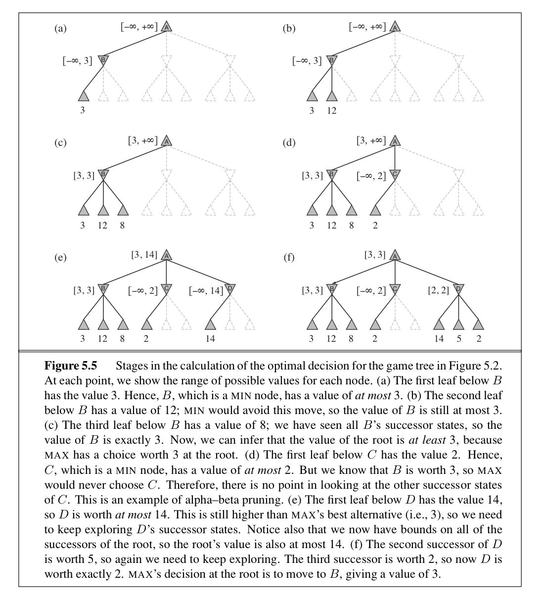
The effectiveness of alpha–beta pruning is highly dependent on the order in which the states are examined. For example, in Figure 5.5(e) and (f), we could not prune any successors of $D$ at all because the worst successors (from the point of view of MIN) were generated first. If the third successor of $D$ had been generated first, we would have been able to prune the other two. This suggests that it might be worthwhile to try to examine first the successors that are likely to be best.

Adding dynamic move-ordering schemes, such as trying first the moves that were found to be best in the past, brings us quite close to the theoretical limit. The past could be the previous move—often the same threats remain—or it could come from previous exploration of the current move. One way to gain information from the current move is with iterative deepening search. First, search 1 ply deep and record the best path of moves. Then search 1 ply deeper, but use the recorded path to inform move ordering.

Imperfect Real-Time Decision

The minimax algorithm generates the entire game search space, whereas the alpha–beta algorithm allows us to prune large parts of it. However, alpha–beta still has to search all the way to terminal states for at least a portion of the search space. This depth is usually not practical, because moves must be made in a reasonable amount of time.

One suggestion is to alter minimax or alpha–beta in two ways: replace the utility function by a heuristic evaluation function EVAL, which estimates the position's utility, and replace the terminal test by a cutoff test that decides when to apply EVAL.

$$\begin{array}{rl}& \text{H-MINIMAX}(s,d)=\\ & \{\begin{array}{ll}\mathrm{EVAL}(s),& \text{CUTOFF-TEST}(s)\\ {\max }_{a\in \mathrm{ACTIONS}(s)}\text{H-MINIMAX}(\mathrm{RESULT}(s,a),d+1),& \mathrm{PLAYER}(s)=\mathrm{MAX}\\ {\min }_{a\in \mathrm{ACTIONS}(s)}\text{H-MINIMAX}(\mathrm{RESULT}(s,a),d+1),& \mathrm{PLAYER}(s)=\mathrm{MIN}\end{array}\end{array}$$

Evaluation functions

Weighted Linear Function

$$\mathrm{EVAL}(s)=\sum _{i=1}^n{w}_i{f}_i(s)$$

Cutting off search

The most basic method is to set a maximum search depth (e.g., "look ahead 6 moves"). The CUTOFF-TEST(state, depth) function returns true when the maximum depth is reached, or when a terminal state (game over) is encountered.

A crucial improvement is to perform the cutoff only when the position is "quiescent." A quiescent position is one where the evaluation score is unlikely to change dramatically in the very near future. For example, in chess, a position with immediate captures available is not quiescent, because the material balance can shift rapidly. A quiescence search extends the search beyond the initial depth limit only for non-quiescent positions, often focusing on specific types of moves (like captures) to resolve the immediate uncertainties.

If a move is considered far better than any other available moves in a given position, this move is then remembered as a singular extension. If this move is available at the search depth limit, the algorithm extends the search to consider this move (so that the search tree may be deeper than expected)

Forward pruning

Some moves at a given node are pruned immediately without further consideration. One approach to forward pruning is beam search: consider only a "beam" of the $n$ best moves (according to the evaluation function) rather than considering all possible moves.

Stochastic Games

Chance nodes are added to the Minimax tree at points where the outcome is determined by chance (e.g., rolling a die, drawing a card, or some other random event). Each chance node has branches representing the possible outcomes of the random event, and each branch is associated with a probability representing the likelihood of that outcome occurring.

$$\text{E-MINIMAX}(s)=\{\begin{array}{ll}\text{UTILITY}(s),& \text{Terminal}(s)\\ {\max }_a\text{E-MINIMAX}(\text{RESULT}(s,a)),& \text{PLAYER}(s)=\text{MAX}\\ {\min }_a\text{E-MINIMAX}(\text{RESULT}(s,a)),& \text{PLAYER}(s)=\text{MIN}\\ {\sum }_{r}P(r)\text{E-MINIMAX}(\text{RESULT(s, a)}),& \text{PLAYER}(s)=\text{CHANCE}\end{array}$$

Evaluation function in stochastic games

Sensitivity to Scale: Unlike deterministic games like chess, where a simple ordering of positions from "better" to "worse" suffices (that is, any partially ordered set that can correctly compare two game state is ok, and we don't need to worry about the absolute value), evaluation functions in stochastic games are highly sensitive to the scale of the assigned values.

The Correct Property: To avoid this sensitivity, the evaluation function must possess a specific property: it must be a positive linear transformation of the probability of winning (or, more generally, of the expected utility) from a given position. This means the evaluation function should be of the form:

$$\text{Evaluation}(s)=a\cdot P(\text{wining from}s)+b$$

where $a>0$ and $b$ are constants.

Partially Observable Games

Card games exemplify stochastic partial observability, where missing information comes from random card distribution.

A simple, but potentially flawed, approach is to average over all possible deals of the hidden cards:

$${\mathrm{argmax}}_a\sum _{s}P(s)\mathrm{MINIMAX}(\mathrm{RESULT}(s,a))$$

where $a$ is the action, $s$ is a deal, $P(s)$ is the probability of that deal. If exact MINIMAX is too costly, H-MINIMAX can be used instead.

Besides, because the number of deals is usually too large, Monte Carlo approximation is used:

$${\mathrm{argmax}}_a\frac{1}{N}\sum _{i=1}^N\mathrm{MINIMAX}\left(\mathrm{RESULT}\left(s_i,a\right)\right)$$

where $N$ is the number of sampled deals and $s_i$ are the sampled deals. Deals are sampled according to their probability $P(s)$, so $P(s)$ doesn't appear explicitly in the formula.

See Also

GAN - Generative Adversarial Nets