Beyond Classical Search

Local Search Algorithms and Optimization Problems

Hill-climbing search

Naive algorithm

The hill-climbing search algorithm (steepest-ascent version) is shown in the code below

def hill_climbing(problem) -> State:
	current = make_node(problem.init_state)
	while (True):
		neighbor = argmax(get_successors(current), 
						  lambda node : node.value)
		if neighbor.value <= current.value:
			return current.state
		current = neighbor

Hill climbing is sometimes called greedy local search because it grabs a good neighbor state without thinking ahead about where to go next. Hill climbing often makes rapid progress toward a solution because it is usually quite easy to improve a bad state. Unfortunately, hill climbing often gets stuck for the following reasons:

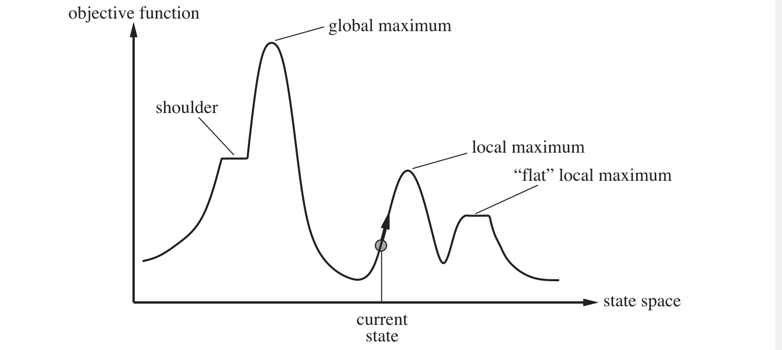
• Local maxima: a local maximum is a peak that is higher than each of its neighboring states but lower than the global maximum.
• Ridges: Ridges result in a sequence of local maxima that is very difficult for greedy algorithms to navigate.
• Plateau: a plateau is a flat area of the state-space landscape. It can be a flat local maximum, from which no uphill exit exists, or a shoulder , form which progress is possible.

Improvements of hill climbing

• Stochastic hill climbing chooses at random from among the uphill moves; the probability of selection can vary with the steepness of the uphill move. This usually converges more slowly than steepest ascent, but in some state landscapes, it finds better solutions.
• First-choice hill climbing implements stochastic hill climbing by generating successors randomly until one is generated that is better than the current state.

Tip

First-choice hill climbing is a good strategy when a state has many (e.g., thousands) of successors

• Random-restart hill climbing conducts a series of hill-climbing searches from randomly generated initial states, until a goal is found. It is trivially complete with probability approaching $1$ , because it will eventually generate a goal state as the initial state.

Simulated annealing

def simulated_annealing(problem, schedule):
    current = make_node(problem.initial_state) 
    for t in range(1, float('inf')): 
        T = schedule(t)
        if T == 0:
            return current
 
        next_state = random.choice(get_successors(current)) 
        delta_e = next_state.value - current.value
 
        if delta_e > 0:
            current = next_state
        else:
            # Accept with probability e^(delta_e / T)
            probability = math.exp(delta_e / T)
            if random.random() < probability:
                current = next_state

Local beam search

The local beam search algorithm keeps track of $k$ states rather than just one. It begins with $k$ randomly generated states. At each step, all the successors of all $k$ states are generated. If any one is a goal, the algorithm halts. Otherwise, it selects the $k$ best successors from the complete list and repeats.

Tip

Unlike random-restart search, in a local beam search, useful information is passed among the parallel search threads.

Local beam search can suffer from a lack of diversity among the $k$ states. A variant called stochastic beam search, analogous to stochastic hill climbing, helps alleviate this problem. Instead of choosing the best $k$ from the pool of candidate successors, stochastic beam search chooses $k$ successors at random, with the probability of choosing a given successor being an increasing function of its value.

Genetic algorithms

A genetic algorithm (or GA) is a variant of stochastic beam search in which successor states are generated by combining two parent states rather than by modifying a single state. The analogy to natural selection is the same as in stochastic beam search, except that now we are dealing with sexual rather than asexual reproduction.

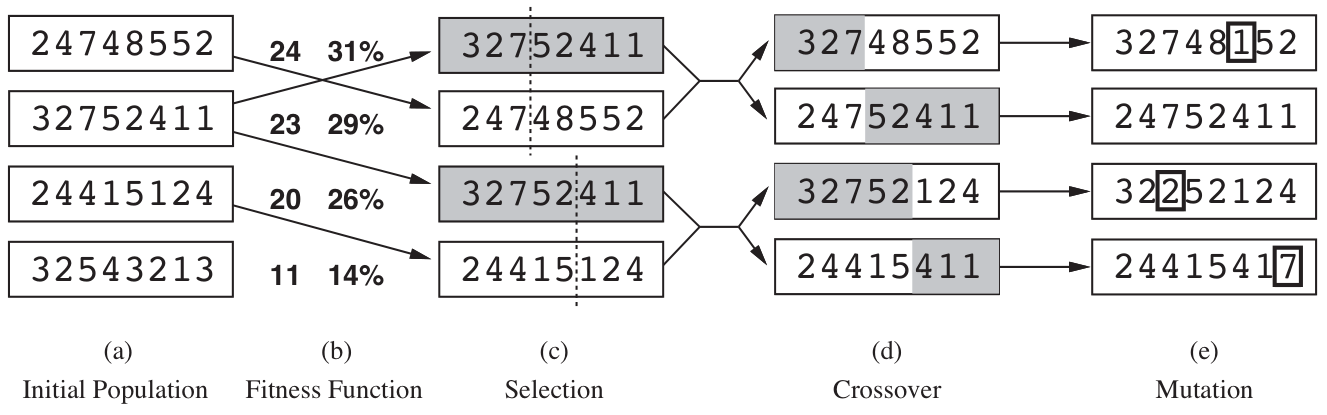
Like beam searchers, GAs begin with a set of $k$ randomly generated states, called the population. Each state, or individual, is represented as a string over a finite alphabet.

In (b), each state is rated by the objective function, or the fitness function. A fitness function should return higher values for better states. In this particular variant of the genetic algorithm, the probability of being chosen for reproducing is directly proportional to the fitness score, and the percentages are shown next to the raw scores.

In (c), two pairs are selected at random of reproduction, in accordance with the probabilities in (b) (so one individual can be selected twice or just be ignored). For each pair to be mated, a crossover point is chosen randomly from the positions in the string.

In (d), the offspring themselves are created by crossing over the parent strings at the crossover point. It is often the case that the population is quite diverse early on in the process, so crossover (like simulated annealing) frequently takes large steps in the state space early in the search process and smaller steps later on when most individuals are quite similar.

In (e), each location is subject to random mutation with a small independent probability.

Local Search in Continuous Spaces

Steepest-ascent hill climbing can be rewritten into

$$\mathbf{x}\leftarrow \mathbf{x}+\alpha \nabla f(\mathbf{x})$$

where $\alpha$ is a small constant often called the step size.

Newton-Raphson method is a general technique for finding roots of functions. It works by computing a new estimate for the root $x$ according to Newton's formula

$$x\leftarrow x-g(x)/g^{\prime }(x)$$

The find a maximum or minimum of $f$, we need to find $\mathbf{x}$ such that the gradient is zero. The update equation can be written in matrix-vector form as

$$\mathbf{x}\leftarrow \mathbf{x}-{\text{H}}_f^{-1}(\mathbf{x})\nabla f(\mathbf{x})$$

where ${\text{H}}_f(\mathbf{x})$ is the Hessian matrix of second derivatives, whose elements $H_{ij}$ are given by $\frac{\partial f}{\partial x_i{x}_j}$.

Searching with Non-Deterministic Actions

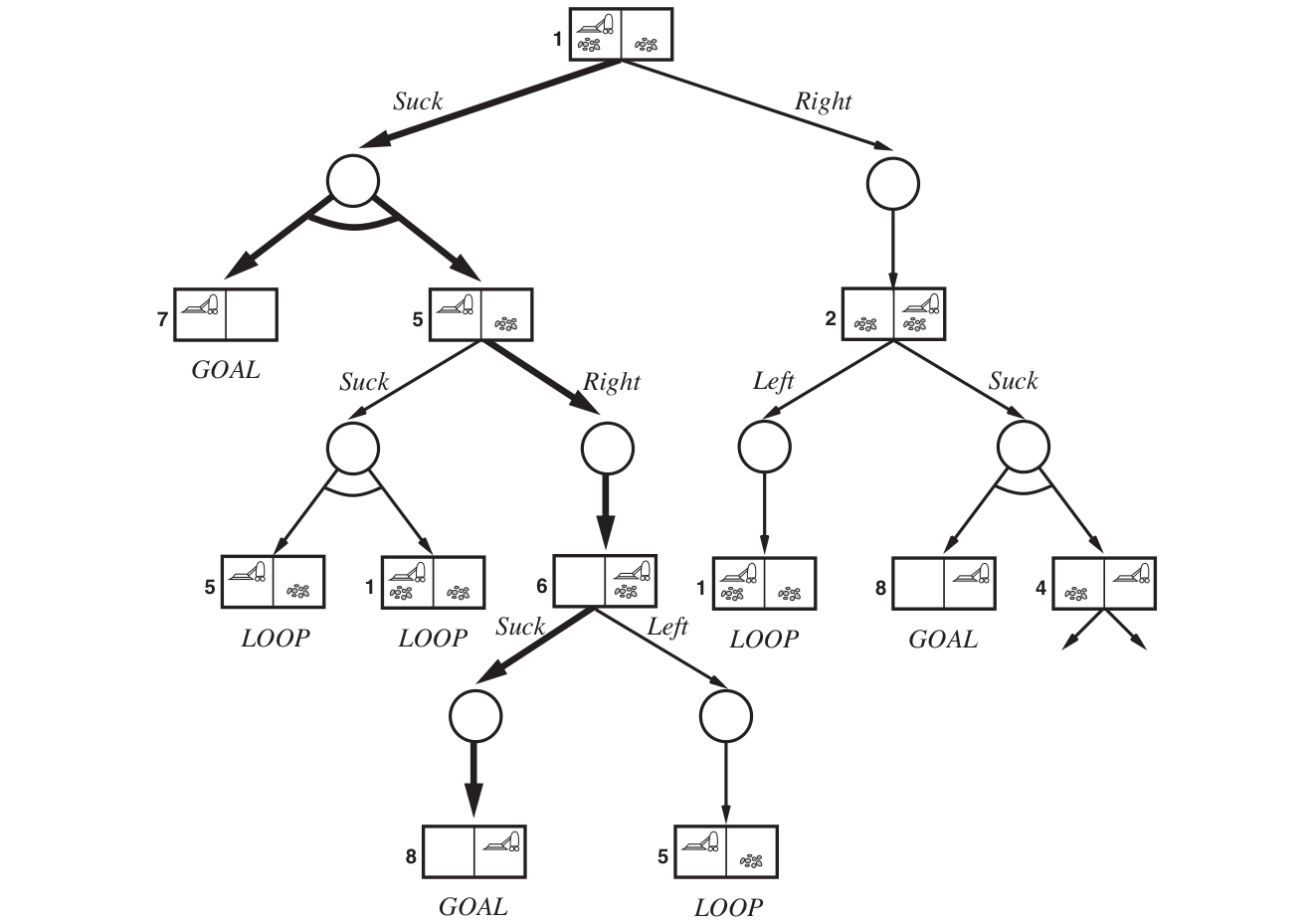
The erratic vacuum world

In the erratic vacuum world, the vacuum cleaner's actions don't always have the expected outcome. Specifically:

• When applied to a dirty square the action cleans the square and sometimes cleans up dirt in an adjacent square, too.
• When applied to a clean square the action sometimes deposits dirt on the carpet.

AND-OR search trees

In a deterministic environment, the only branching is introduced by the agents' own choices in each state. We call these nodes OR nodes. In a nondeterministic environment, branching is also introduced by the environment’s choice of outcome for each action. We call these nodes AND nodes.

def AND_OR_GRAPH_SEARCH(problem):
    """
    Searches for a conditional plan in an AND-OR graph.
 
    Args:
        problem: A problem definition object with the following methods:
            INITIAL_STATE: Returns the initial state of the problem.
            GOAL_TEST(state): Returns True if the state is a goal state, False otherwise.
            ACTIONS(state): Returns a list of possible actions from the given state.
            RESULTS(state, action): Returns a list of possible resulting states after
                taking the given action in the given state.
    
    Returns:
        A conditional plan (a list of actions and conditional branches), or
        "failure" if no plan is found.
    """
    return OR_SEARCH(problem.INITIAL_STATE, problem, [])
 
def OR_SEARCH(state, problem, path):
    """
    Searches for a plan from the current state in an OR node.
 
    Args:
        state: The current state.
        problem: The problem definition object.
        path: A list of states representing the path from the initial state to the current state.
 
    Returns:
        A conditional plan, or "failure".
    """
    if problem.GOAL_TEST(state):
        return []  # The empty plan
 
    if state in path:
        return "failure"
 
    for action in problem.ACTIONS(state):
        resulting_states = problem.RESULTS(state, action)
        plan = AND_SEARCH(resulting_states, problem, [state] + path)
 
        if plan != "failure":
            return [action] + [plan]  # Add action to the beginning of the plan
    
    return "failure"
 
def AND_SEARCH(states, problem, path):
    """
    Searches for a plan that works in all possible resulting states (AND node).
 
    Args:
        states: A list of possible resulting states.
        problem: The problem definition object.
        path: A list of states representing the path.
 
    Returns:
        A conditional plan, or "failure".
    """
    plans = []
    for s in states:
        plan_i = OR_SEARCH(s, problem, path)
        plans.append(plan_i)
        if plan_i == "failure":
            return "failure"
 
    # Construct the conditional plan
    conditional_plan = "if "
    for i in range(len(states)):
        if i > 0:
             conditional_plan += " else if "
        conditional_plan += str(states[i]) + " then " + str(plans[i])
    conditional_plan += " else " + str(plans[-1]) 
    return conditional_plan
 

Searching with Partial Observations

We now turn to the problem of partial observability, where the agents's precepts do not suffice to pin down the exact state. The key concept required for solving partially observable problems is the belief state.

Searching with no observation

When the agent's precepts provide no information at all, we have what is called a sensor-less problem or sometimes a conformant problem.

We can make a sensor-less version of the vacuum world. Assume that the agent knows the geography of its world, but doesn't know its location or the distribution of dirt. In that case, its initial state could be any element of the set $\left\{1,2,\dots ,8\right\}$. Now, consider what happens if it tries the action $\mathrm{RIGHT}$. This will cause it to be in one of the states $\left\{2,4,6,8\right\}$, thus the agent now has more information.

To solve sensor-less problems, we search in the space of belief states rather than physical states. Notice that in belief-state space, the problem is fully observable because the agent always knows its own belief state.

Suppose the underlying physical problem $P$ is defined by ${\mathrm{ACTIONS}}_P,{\mathrm{RESULT}}_P,{\mathrm{GOAL}-\mathrm{TEST}}_P$ and ${\mathrm{STEP}-\mathrm{COST}}_p$. Then we can define the corresponding sensor-less problem as follows:

• Belief states: The entire belief-state space contains every possible set of physical states. If $P$ has $N$ states, then the sensor-less problems has up to $2^N$ states, although many may be unreachable from the initial state. (For each of these $N$ states, the agent either believes it could be in that state, or it doesn't. This is a binary (two-option) choice.)
• Initial state: Typically the set of all states in $P$
• Actions: Suppose the agent is in belief state $b=\left\{s_1,s_2\right\}$, but ${\mathrm{ACTIONS}}_P(s_1)\ne {\mathrm{ACTIONS}}_P(s_2)$; then the agent is unsure of which actions are legal. If we assume that illegal actions have no effect on the environment, then it is safe to take the union of all the actions in any of the physical states in the current belief state $b$:

$$\mathrm{ACTIONS}(b)=\bigcup _{s\in b}{\mathrm{ACTIONS}}_P(s)$$

On the other hand, if an illegal action might be the end of the world, it is safer to allow only the intersection, that is, the set of actions legal in all the states.

• Transition model: The agent doesn’t know which state in the belief state is the right one; so as far as it knows, it might get to any of the states resulting from applying the action to one of the physical states in the belief state. For deterministic actions, the set of states that might be reached is

$$b^{\prime }=\left\{s^{\prime }\mid s^{\prime }={\mathrm{RESULT}}_P(s,a),s\in b\right\}$$

With non-determinism, we have

$$b^{\prime }=\left\{s^{\prime }\mid s^{\prime }\in {\mathrm{RESULT}}_P(s,a),s\in b\right\}$$

• Goal test: The agent wants a plan that is sure to work, which means that a belief state satisfies the goal only if all the physical states in it satisfy ${\mathrm{GOAL}-\mathrm{TEST}}_P$.
• Path cost: If the same action can have different costs in different states, then the cost of taking an action in a given belief state could be one of several values. For now we assume that the cost of an action is the same in all states and so can be transferred directly from the underlying physical problem.

For the algorithm to solve the problem, one crucial issue is that the belief-state space can grow exponentially larger than the actual environment, making searches computationally demanding. Incremental search algorithms mitigate this by constructing solutions step-by-step, rather than exploring the entire belief-state space at once. They begin with a smaller set of possible states, attempt to find a plan for this subset, and expand the set if the plan fails for other potential states. This process continues until a plan is found that works for all possibilities within the belief state. This approach allows for early detection of unsolvable problems, as failures within smaller subsets indicate a lack of solution for the entire belief state. By avoiding full exploration of the belief-state space, these algorithms improve efficiency.

Searching with observations

Solving partially observable problems

An agent for partially observable environments

Online Search Agents and Unknown Environments

So far we have concentrated on agents that use offline search algorithms. They compute a complete solution before setting foot in the real world and then execute the solution. In contrast, an online search agent interleaves computation and action: first it takes an action, then it observes the environment and computes the next action.

Online search is a necessary idea for unknown environments, where the agent does not know what states exist or what its actions do. In this state of ignorance, the agent faces an exploration problem and must use its actions as experiments in order to learn enough to make deliberation worthwhile.

Online search problems

Competitive Ratio The total path cost of the path that the agent actually travels / The actual shortest path.

The idea ratio is 1 (same as the off-line case)

Online search agents

Learning real-time A*

def lrta_star_agent(s_prime, goal_test, actions, c, h):
    """
    LRTA* agent implementation.
 
    Args:
        s_prime: Current state (percept).
        goal_test: Function to test if a state is the goal.
        actions: Function to get available actions from a state.
        c: Cost function c(s, a, s').
        h: Heuristic function h(s).
 
    Returns:
        An action.
    """
 
    if not hasattr(lrta_star_agent, "result"):
        lrta_star_agent.result = {}  # Initialize result table (state, action -> next state)
        lrta_star_agent.H = {}      # Initialize heuristic table (state -> cost estimate)
        lrta_star_agent.s = None      # Initialize previous state
        lrta_star_agent.a = None      # Initialize previous action
 
    if goal_test(s_prime):
        return "stop"
 
    if s_prime not in lrta_star_agent.H:
        lrta_star_agent.H[s_prime] = h(s_prime)
 
    if lrta_star_agent.s is not None:
        lrta_star_agent.result[(lrta_star_agent.s, lrta_star_agent.a)] = s_prime
        lrta_star_agent.H[lrta_star_agent.s] = min(
            lrta_star_cost(lrta_star_agent.s, b, lrta_star_agent.result.get((lrta_star_agent.s, b)), lrta_star_agent.H, c, h)
            for b in actions(lrta_star_agent.s)
        )
 
    best_action = min(
        actions(s_prime),
        key=lambda b: lrta_star_cost(s_prime, b, lrta_star_agent.result.get((s_prime, b)), lrta_star_agent.H, c, h)
    )
 
    lrta_star_agent.a = best_action
    lrta_star_agent.s = s_prime
    return best_action
 
def lrta_star_cost(s, a, s_prime, H, c, h):
    """
    LRTA* cost estimate function.
 
    Args:
        s: Current state.
        a: Action.
        s_prime: Next state.
        H: Heuristic table.
        c: Cost function.
        h: Heuristic function.
 
    Returns:
        Cost estimate.
    """
    if (s,a) not in lrta_star_agent.result:
        return h(s)
    else:
        return c(s, a, s_prime) + H[s_prime]
 
# Example usage (simplified grid world):
 
def goal_test_example(state):
    return state == (2, 2)
 
def actions_example(state):
    possible_actions = []
    if state[0] > 0: possible_actions.append("left")
    if state[0] < 2: possible_actions.append("right")
    if state[1] > 0: possible_actions.append("up")
    if state[1] < 2: possible_actions.append("down")
    return possible_actions
 
def c_example(s, a, s_prime):
    return 1  # Constant cost for all actions
 
def h_example(state):
    return abs(state[0] - 2) + abs(state[1] - 2)  # Manhattan distance heuristic
 
# Simulation:
current_state = (0, 0)
for _ in range(10):  # Run for a few steps
    action = lrta_star_agent(current_state, goal_test_example, actions_example, c_example, h_example)
    print(f"Current state: {current_state}, Action: {action}")
    if action == "stop":
      break
    if action == "left": current_state = (current_state[0]-1, current_state[1])
    elif action == "right": current_state = (current_state[0]+1, current_state[1])
    elif action == "up": current_state = (current_state[0], current_state[1]-1)
    elif action == "down": current_state = (current_state[0], current_state[1]+1)