Denoising Diffusion Probabilistic Models (DDPM)

Overview

Diffusion models are incremental updates where the assembly of the whole gives us the encoder-decoder structure. The transition from one state to another is realized by a denoiser.

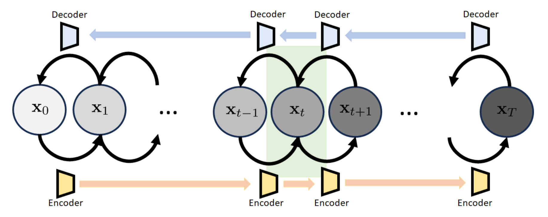The model whose structure is shown above is called the variational diffusion model (VDM). The model has a sequence of states ${\mathbf{x}}_0,{\mathbf{x}}_1,\dots ,{\mathbf{x}}_T$

• ${\mathbf{x}}_0$: the original image, which is the same as $\mathbf{x}$ in VAE
• ${\mathbf{x}}_T$: the latent variable, which is the same as $\mathbf{z}$ in VAE, and we want to make it Gaussian: ${\mathbf{x}}_T\sim \mathcal{N}(0,\text{I})$
• ${\mathbf{x}}_1,\dots ,{\mathbf{x}}_{T-1}$: the intermediate states, which are also the latent variables, but not white Gaussian

Building Blocks

Transition Block

The $t$-th transition block consists of three states ${\mathbf{x}}_{t-1},{\mathbf{x}}_t$ and ${\mathbf{x}}_{t+1}$. There are two possible paths to get to state ${\mathbf{x}}_t$

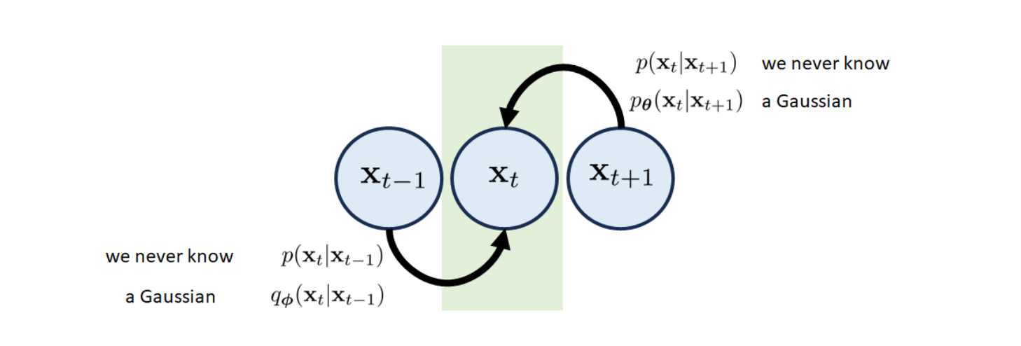
• The forward transition that goes from ${\mathbf{x}}_{t-1}$ to ${\mathbf{x}}_t$. The associated transition distribution is $p({\mathbf{x}}_t|{\mathbf{x}}_{t-1})$. That is, we can sample ${\mathbf{x}}_t$ from $p({\mathbf{x}}_t|{\mathbf{x}}_{t-1})$ for given ${\mathbf{x}}_{t-1}$. Just like VAE, we do not have access to $p({\mathbf{x}}_t|{\mathbf{x}}_{t-1})$, so we will approximate it by a Gaussian $q_{\mathbf{\varphi }}({\mathbf{x}}_t|{\mathbf{x}}_{t-1})$
• The reverse transition goes from ${\mathbf{x}}_{t+1}$ to ${\mathbf{x}}_t$. Again, we never know $p({\mathbf{x}}_{t+1}|{\mathbf{x}}_t)$ so we use another Gaussian $p_{\mathbf{\theta }}({\mathbf{x}}_{t+1}|{\mathbf{x}}_t)$ to approximate it

Initial Block

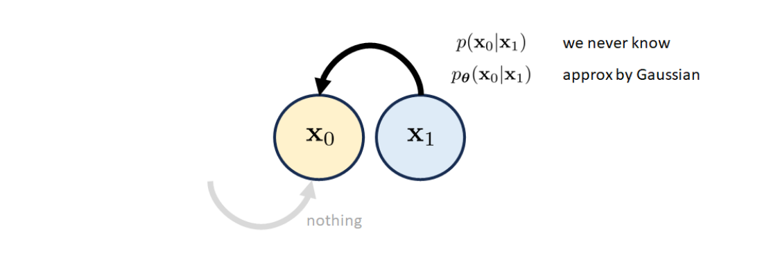Just without forward path.

Final Block

Just without reverse path, and the final variable ${\mathbf{x}}_T$ should be Gaussian

Transition Distribution

In a denoising diffusion probabilistic model, the transition distribution $q_{\mathbf{\varphi }}({\mathbf{x}}_t|{\mathbf{x}}_{t-1})$ is defined (yes, this is defined, not derived by training) as

$$q_{\mathbf{\varphi }}({\mathbf{x}}_t|{\mathbf{x}}_{t-1})=\mathcal{N}({\mathbf{x}}_t\mid \sqrt{{\alpha }_t}{\mathbf{x}}_{t-1},(1-{\alpha }_t)\text{I})$$

That is, the transition distribution is a Gaussian with mean $\sqrt{{\alpha }_t}{\mathbf{x}}_t$ and variance $1-{\alpha }_t$. The choice of the scaling factor $\sqrt{{\alpha }_t}$ is to make sure that the variance magnitude is preserved so that it will not explode and vanish after many iterations

Tip

$\sqrt{{\alpha }_t}$ and $1-{\alpha }_t$ are chosen so that the distribution of ${\mathbf{x}}_t$ will become $\mathcal{N}(0,\text{I})$ when $t$ is large enough.

From this transition distribution, we can obtain how ${\mathbf{x}}_t$ will be distributed if we are given ${\mathbf{x}}_0$:

$$q_{\mathbf{\varphi }}({\mathbf{x}}_t|{\mathbf{x}}_0)=\mathcal{N}({\mathbf{x}}_t\mid \sqrt{{\bar{\alpha }}_t}{\mathbf{x}}_0,(1-{\bar{\alpha }}_t)\text{I})$$

where ${\bar{\alpha }}_t={\prod }_{i=1}^t{\alpha }_i$

Evidence Lower Bound

Like in VAE, we need to maximize the ELBO to train the model, the ELBO in variational diffusion model is

$$\boxed{\begin{array}{rl}{\mathrm{ELBO}}_{\mathbf{\varphi },\mathbf{\theta }}(\mathbf{x})& ={\mathbb{E}}_{q_{\mathbf{\varphi }}({\mathbf{x}}_1|{\mathbf{x}}_0)}\left[\log \underset{\text{how good the initial block is}}{\underbrace{p_{\mathbf{\theta }}({\mathbf{x}}_0|{\mathbf{x}}_1)}}\right]\\ & -{\mathbb{E}}_{q_{\mathbf{\varphi }}({\mathbf{x}}_{T-1}|{\mathbf{x}}_0)}\left[\underset{\text{how good the final block is}}{\underbrace{{\mathbb{D}}_{\mathrm{KL}}\left(q_{\mathbf{\varphi }}({\mathbf{x}}_T|{\mathbf{x}}_{T-1})\Vert p({\mathbf{x}}_T)\right)}}\right]\\ & -\sum _{t=1}^{T-1}{\mathbb{E}}_{q_{\mathbf{\varphi }}}({\mathbf{x}}_{t-1},{\mathbf{x}}_{t+1}|{\mathbf{x}}_0)\left[\underset{\text{how good the transition blocks are}}{\underbrace{{\mathbb{D}}_{\mathrm{KL}}\left(q_{\mathbf{\varphi }}({\mathbf{x}}_t|{\mathbf{x}}_{t-1})\Vert p_{\mathbf{\theta }}({\mathbf{x}}_t|{\mathbf{x}}_{t+1})\right)}}\right]\end{array}}$$

The ELBO here consists of three components:

• Reconstruction. This term is based on the initial block. We use the log-likelihood $p_{\mathbf{\theta }}({\mathbf{x}}_0|{\mathbf{x}}_1)$ to measure how good the neural network associated with $p_{\mathbf{\theta }}$ can recover from the latent variable ${\mathbf{x}}_1$. The expectation is taken with respect to the samples drawn from $q_{\mathbf{\varphi }}({\mathbf{x}}_1|{\mathbf{x}}_0)$ during the encoding process.
• Prior Matching. The prior matching term is based on the final block. We use KL divergence to measure the difference between $q_{\mathbf{\varphi }}({\mathbf{x}}_T|{\mathbf{x}}_{T-1})$ and $p({\mathbf{x}}_T)$. We want how ${\mathbf{x}}_T$ is generated, $q_{\mathbf{\varphi }}({\mathbf{x}}_T|{\mathbf{x}}_{T-1})$, to be as close to our desired $p({\mathbf{x}}_T)$, namely $\mathcal{N}(0,\text{I})$, as possible. The samples here are ${\mathbf{x}}_{T-1}$ which are drawn from $q_{\mathbf{\varphi }}({\mathbf{x}}_{T-1}|{\mathbf{x}}_0)$ because this distribution provides the forward sample generation process.
• Consistency. The consistency term is based on the transition blocks, which uses the KL divergence to measure the deviation between the forward path and the reverse path.

Proof of ELBO

Recall by the definition of ELBO, we have

$$\log p(x)=\mathrm{ELBO}(x)+{\mathbb{D}}_{\mathrm{KL}}(q_{\varphi }(z|x)\Vert p(z|x))$$

This means that ELBO is an evidence lower bound for $\log p(x)$, and now we try to estimate it. Let's define the notation: ${\mathbf{x}}_{0:T}=\left\{{\mathbf{x}}_0,\dots ,{\mathbf{x}}_T\right\}$ means the collection of all state variable from $t=0$ to $t=T$. We recall that the prior distribution $p(\mathbf{x})$ is the distribution of the image ${\mathbf{x}}_0$, so

$$\begin{array}{rl}\log p(\mathbf{x})& =\log p({\mathbf{x}}_0)\\ & =\log \int p({\mathbf{x}}_{0:T})\mathrm{d}{\mathbf{x}}_{1:T}\\ & =\log \int p({\mathbf{x}}_{0:T})\frac{q_{\mathbf{\varphi }}({\mathbf{x}}_{1:T}|{\mathbf{x}}_0)}{q_{\mathbf{\varphi }}({\mathbf{x}}_{1:T}|{\mathbf{x}}_0)}\mathrm{d}{\mathbf{x}}_{1:T}\\ & =\log \int q_{\mathbf{\varphi }}({\mathbf{x}}_{1:T}|{\mathbf{x}}_0)\left[\frac{p({\mathbf{x}}_{0:T})}{q_{\mathbf{\varphi }}({\mathbf{x}}_{1:T}|{\mathbf{x}}_0)}\right]\mathrm{d}{\mathbf{x}}_{1:T}\\ & =\log {\mathbb{E}}_{q_{\mathbf{\varphi }}({\mathbf{x}}_{1:T}|{\mathbf{x}}_0)}\left[\frac{p({\mathbf{x}}_{0:T})}{q_{\mathbf{\varphi }}({\mathbf{x}}_{1:T}|{\mathbf{x}}_0)}\right]\end{array}$$

With Jensen's inequality, which states that for any random variable $X$ and any concave function $f$, it holds that $f(\mathbb{E}[X]\ge \mathbb{E}[f(X)]$, so we have

$$\begin{array}{rl}\log p(\mathbf{x})& =\log {\mathbb{E}}_{q_{\mathbf{\varphi }}({\mathbf{x}}_{1:T}|{\mathbf{x}}_0)}\left[\frac{p({\mathbf{x}}_{0:T})}{q_{\mathbf{\varphi }}({\mathbf{x}}_{1:T}|{\mathbf{x}}_0)}\right]\\ & \ge {\mathbb{E}}_{q_{\mathbf{\varphi }}({\mathbf{x}}_{1:T}|{\mathbf{x}}_0)}\left[\log \frac{p({\mathbf{x}}_{0:T})}{q_{\mathbf{\varphi }}({\mathbf{x}}_{1:T}|{\mathbf{x}}_0)}\right]\\ & ={\mathbb{E}}_{q_{\mathbf{\varphi }}({\mathbf{x}}_{1:T}|{\mathbf{x}}_0)}\left[\log \frac{p({\mathbf{x}}_T)p({\mathbf{x}}_0|{\mathbf{x}}_1){\prod }_{t=2}^{T}p({\mathbf{x}}_{t-1}|{\mathbf{x}}_t)}{q_{\mathbf{\varphi }}({\mathbf{x}}_T|{\mathbf{x}}_{T-1}){\prod }_{t=1}^{T-1}{q}_{\mathbf{\varphi }}({\mathbf{x}}_t|{\mathbf{x}}_{t-1})}\right](\text{by Markov property})\\ & ={\mathbb{E}}_{q_{\mathbf{\varphi }}({\mathbf{x}}_{1:T}|{\mathbf{x}}_0)}\left[\log \frac{p({\mathbf{x}}_T)p({\mathbf{x}}_0|{\mathbf{x}}_1){\prod }_{t=1}^{T-1}p({\mathbf{x}}_t|{\mathbf{x}}_{t+1})}{q_{\mathbf{\varphi }}({\mathbf{x}}_T|{\mathbf{x}}_{T-1}){\prod }_{t=1}^{T-1}{q}_{\mathbf{\varphi }}({\mathbf{x}}_t|{\mathbf{x}}_{t-1})}\right](\text{shift}t\text{to}t+1)\\ & ={\mathbb{E}}_{q_{\mathbf{\varphi }}({\mathbf{x}}_{1:T}|{\mathbf{x}}_0)}\left[\log \frac{p({\mathbf{x}}_T)p({\mathbf{x}}_0|{\mathbf{x}}_1)}{q_{\mathbf{\varphi }}({\mathbf{x}}_T|{\mathbf{x}}_{T-1})}\right]+{\mathbb{E}}_{q_{\mathbf{\varphi }}({\mathbf{x}}_{1:T}|{\mathbf{x}}_0)}\left[\log \prod _{t=1}^{T-1}\frac{p({\mathbf{x}}_t|{\mathbf{x}}_{t+1})}{q_{\mathbf{\varphi }}({\mathbf{x}}_t|{\mathbf{x}}_{t-1})}\right]\end{array}$$

where the first item can be decomposed into two parts:

$$\begin{array}{rl}{\mathbb{E}}_{q_{\mathbf{\varphi }}({\mathbf{x}}_{1:T}|{\mathbf{x}}_0)}\left[\log \frac{p({\mathbf{x}}_T)p({\mathbf{x}}_0|{\mathbf{x}}_1)}{q_{\mathbf{\varphi }}({\mathbf{x}}_T|{\mathbf{x}}_{T-1})}\right]& ={\mathbb{E}}_{q_{\mathbf{\varphi }}({\mathbf{x}}_{1:T}|{\mathbf{x}}_0)}\left[\log p({\mathbf{x}}_0|{\mathbf{x}}_1)\right]\\ & +{\mathbb{E}}_{q_{\mathbf{\varphi }}({\mathbf{x}}_{1:T}|{\mathbf{x}}_0)}\left[\log \frac{p({\mathbf{x}}_T)}{q_{\mathbf{\varphi }}({\mathbf{x}}_T|{\mathbf{x}}_{T-1})}\right]\\ & =\underset{\text{Reconstruction}}{\underbrace{{\mathbb{E}}_{q_{\mathbf{\varphi }}({\mathbf{x}}_1|{\mathbf{x}}_0)}\left[\log p({\mathbf{x}}_0|{\mathbf{x}}_1)\right]}}\\ & -\underset{\text{Prior Matching}}{\underbrace{{\mathbb{E}}_{q_{\mathbf{\varphi }}({\mathbf{x}}_{T-1},{\mathbf{x}}_T|{\mathbf{x}}_0)}\left[{\mathbb{D}}_{\mathrm{KL}}(q_{\mathbf{\varphi }}({\mathbf{x}}_T|{\mathbf{x}}_{T-1})\Vert p({\mathbf{x}}_T))\right]}}\end{array}$$

and the second term is

$$\begin{array}{rl}{\mathbb{E}}_{q_{\mathbf{\varphi }}({\mathbf{x}}_{1:T}|{\mathbf{x}}_0)}\left[\log \prod _{t=1}^{T-1}\frac{p({\mathbf{x}}_t|{\mathbf{x}}_{t+1})}{q_{\mathbf{\varphi }}({\mathbf{x}}_t|{\mathbf{x}}_{t-1})}\right]& =\sum _{t=1}^{T-1}{\mathbb{E}}_{q_{\mathbf{\varphi }}({\mathbf{x}}_{1:T}|{\mathbf{x}}_0)}\left[\log \frac{p({\mathbf{x}}_t|{\mathbf{x}}_{t+1})}{q_{\mathbf{\varphi }}({\mathbf{x}}_t|{\mathbf{x}}_{t-1})}\right]\\ & =\sum _{t=1}^{T-1}{\mathbb{E}}_{q_{\mathbf{\varphi }}({\mathbf{x}}_{t-1},{\mathbf{x}}_t,{\mathbf{x}}_{t+1}|{\mathbf{x}}_0)}\left[\log \frac{p({\mathbf{x}}_t|{\mathbf{x}}_{t+1})}{q_{\mathbf{\varphi }}({\mathbf{x}}_t|{\mathbf{x}}_{t-1})}\right]\\ & =-\underset{\text{Consistency}}{\underbrace{\sum _{t=1}^{T-1}{\mathbb{E}}_{q_{\mathbf{\varphi }}({\mathbf{x}}_{t-1},{\mathbf{x}}_{t+1}|{\mathbf{x}}_0)}\left[{\mathbb{D}}_{\mathrm{KL}}\left(q_{\mathbf{\varphi }}({\mathbf{x}}_t|{\mathbf{x}}_{t-1})\Vert p({\mathbf{x}}_t|{\mathbf{x}}_{t+1})\right)\right]}}\end{array}$$

where the last line used:

$$\begin{array}{rl}{q}_{\mathbf{\varphi }}({\mathbf{x}}_{t-1},{\mathbf{x}}_t,{\mathbf{x}}_{t+1}|{\mathbf{x}}_0)& =q_{\mathbf{\varphi }}({\mathbf{x}}_{t-1},{\mathbf{x}}_t,{\mathbf{x}}_{t+1}|{\mathbf{x}}_{t-1},{\mathbf{x}}_{t+1},{\mathbf{x}}_0)\cdot q_{\mathbf{\varphi }}({\mathbf{x}}_{t-1},{\mathbf{x}}_{t+1}|{\mathbf{x}}_0)\\ & =q_{\mathbf{\varphi }}({\mathbf{x}}_t|{\mathbf{x}}_{t-1},{\mathbf{x}}_{t+1},{\mathbf{x}}_0)\cdot q_{\mathbf{\varphi }}({\mathbf{x}}_{t-1},{\mathbf{x}}_{t+1}|{\mathbf{x}}_0)\\ & =q_{\mathbf{\varphi }}({\mathbf{x}}_t|{\mathbf{x}}_{t-1})\cdot q_{\mathbf{\varphi }}({\mathbf{x}}_{t-1},{\mathbf{x}}_{t+1}|{\mathbf{x}}_0)\text{(by Markov properity)}\end{array}$$

Rewrite the Consistency Term

If we want to maximize the ELBO above, we need to handle two opposite directions: $q_{\mathbf{\varphi }}({\mathbf{x}}_t|{\mathbf{x}}_{t-1})$ and $p_{\mathbf{\theta }}({\mathbf{x}}_t|{\mathbf{x}}_{t+1})$ in the consistency and prior matching term. However, we could use Bayes' Theorem to avoid this:

$$q({\mathbf{x}}_t|{\mathbf{x}}_{t-1})=\frac{q({\mathbf{x}}_{t-1}|{\mathbf{x}}_t)q({\mathbf{x}}_t)}{q({\mathbf{x}}_{t-1})}⟹q({\mathbf{x}}_t|{\mathbf{x}}_{t-1},{\mathbf{x}}_0)=\frac{q({\mathbf{x}}_{t-1}|{\mathbf{x}}_t,{\mathbf{x}}_0)q({\mathbf{x}}_t|{\mathbf{x}}_0)}{q({\mathbf{x}}_{t-1}|{\mathbf{x}}_0)}$$

The "$⟹$" step conditions the probability on ${\mathbf{x}}_0$ since we are primarily concerned with generating the data ${\mathbf{x}}_0$ in denoising diffusion models. By introducing this conditioning on ${\mathbf{x}}_0$, we aim to incorporate information about the full data trajectory when estimating $q({\mathbf{x}}_t|{\mathbf{x}}_{t-1},{\mathbf{x}}_0)$. For diffusion models, the reverse process can now be estimated with a noise predictor that approximates the distribution of ${\mathbf{x}}_{t-1}$ given ${\mathbf{x}}_t$. The ELBO maximization will involve minimizing the KL divergence between the learned model $p_{\mathbf{\theta }}$ and the posterior $q_{\mathbf{\varphi }}({\mathbf{x}}_{t-1}|{\mathbf{x}}_t,{\mathbf{x}}_0)$, that is, the new consistency term.

To be specific, starting from the Jenson inequality in section Proof of ELBO above:

$$\begin{array}{rl}\log p(\mathbf{x})& \ge {\mathbb{E}}_{q_{\mathbf{\varphi }}({\mathbf{x}}_{1:T}|{\mathbf{x}}_0)}\left[\log \frac{p({\mathbf{x}}_{0:T})}{q_{\mathbf{\varphi }}({\mathbf{x}}_{1:T}|{\mathbf{x}}_0)}\right]\\ & ={\mathbb{E}}_{q_{\mathbf{\varphi }}({\mathbf{x}}_{1:T}|{\mathbf{x}}_0)}\left[\log \frac{p({\mathbf{x}}_T)p({\mathbf{x}}_0|{\mathbf{x}}_1){\prod }_{t=2}^{T}p({\mathbf{x}}_{t-1}|{\mathbf{x}}_t)}{q_{\mathbf{\varphi }}({\mathbf{x}}_1|{\mathbf{x}}_0){\prod }_{t=2}^T{q}_{\mathbf{\varphi }}({\mathbf{x}}_t|{\mathbf{x}}_{t-1},{\mathbf{x}}_0)}\right]\\ & ={\mathbb{E}}_{q_{\mathbf{\varphi }}({\mathbf{x}}_{1:T}|{\mathbf{x}}_0)}\left[\log \frac{p({\mathbf{x}}_T)p({\mathbf{x}}_0|{\mathbf{x}}_1)}{q_{\mathbf{\varphi }}({\mathbf{x}}_1|{\mathbf{x}}_0)}\right]+{\mathbb{E}}_{q_{\mathbf{\varphi }}({\mathbf{x}}_{1:T}|{\mathbf{x}}_0)}\left[\log \prod _{t=2}^T\frac{p({\mathbf{x}}_{t-1}|{\mathbf{x}}_t)}{q_{\mathbf{\varphi }}({\mathbf{x}}_t|{\mathbf{x}}_{t-1},{\mathbf{x}}_0)}\right]\end{array}$$

And now we can apply Bayes' Theorem in the second term

$$\begin{array}{rl}\prod _{t=2}^T\frac{p({\mathbf{x}}_{t-1}|{\mathbf{x}}_t)}{q_{\mathbf{\varphi }}({\mathbf{x}}_t|{\mathbf{x}}_{t-1},{\mathbf{x}}_0)}& =\prod _{t=2}^T\frac{p({\mathbf{x}}_{t-1}|{\mathbf{x}}_t)}{\frac{q_{\mathbf{\varphi }}({\mathbf{x}}_{t-1}|{\mathbf{x}}_t,{\mathbf{x}}_0)q_{\mathbf{\varphi }}({\mathbf{x}}_t|{\mathbf{x}}_0)}{q_{\mathbf{\varphi }}({\mathbf{x}}_{t-1}|{\mathbf{x}}_0)}}\\ & =\prod _{t=2}^T\frac{p({\mathbf{x}}_{t-1}|{\mathbf{x}}_t)}{q_{\mathbf{\varphi }}({\mathbf{x}}_{t-1}|{\mathbf{x}}_t,{\mathbf{x}}_0)}\times \prod _{t=2}^T\frac{q_{\mathbf{\varphi }}({\mathbf{x}}_{t-1}|{\mathbf{x}}_0)}{q_{\mathbf{\varphi }}({\mathbf{x}}_t|{\mathbf{x}}_0)}\\ & =\prod _{t=2}^T\frac{p({\mathbf{x}}_{t-1}|{\mathbf{x}}_t)}{q_{\mathbf{\varphi }}({\mathbf{x}}_{t-1}|{\mathbf{x}}_t,{\mathbf{x}}_0)}\times \frac{q_{\mathbf{\varphi }}({\mathbf{x}}_1|{\mathbf{x}}_0)}{q_{\mathbf{\varphi }}({\mathbf{x}}_T|{\mathbf{x}}_0)}\end{array}$$

Then we could continue the inequality

$$\begin{array}{rl}\log p(\mathbf{x})& \ge {\mathbb{E}}_{q_{\mathbf{\varphi }}({\mathbf{x}}_{1:T}|{\mathbf{x}}_0)}\left[\log \frac{p({\mathbf{x}}_T)p({\mathbf{x}}_0|{\mathbf{x}}_1)}{q_{\mathbf{\varphi }}({\mathbf{x}}_1|{\mathbf{x}}_0)}\right]+{\mathbb{E}}_{q_{\mathbf{\varphi }}({\mathbf{x}}_{1:T}|{\mathbf{x}}_0)}\left[\log \prod _{t=2}^T\frac{p({\mathbf{x}}_{t-1}|{\mathbf{x}}_t)}{q_{\mathbf{\varphi }}({\mathbf{x}}_t|{\mathbf{x}}_{t-1},{\mathbf{x}}_0)}\right]\\ & ={\mathbb{E}}_{q_{\mathbf{\varphi }}({\mathbf{x}}_{1:T}|{\mathbf{x}}_0)}\left[\log \frac{p({\mathbf{x}}_T)p({\mathbf{x}}_0|{\mathbf{x}}_1)}{q_{\mathbf{\varphi }}({\mathbf{x}}_1|{\mathbf{x}}_0)}+\log \frac{q_{\mathbf{\varphi }}({\mathbf{x}}_1|{\mathbf{x}}_0)}{q_{\mathbf{\varphi }}({\mathbf{x}}_T|{\mathbf{x}}_0)}\right]\\ & +{\mathbb{E}}_{q_{\mathbf{\varphi }}({\mathbf{x}}_{1:T}|{\mathbf{x}}_0)}\left[\log \prod _{t=2}^T\frac{p({\mathbf{x}}_{t-1}|{\mathbf{x}}_t)}{q_{\mathbf{\varphi }}({\mathbf{x}}_{t-1}|{\mathbf{x}}_t,{\mathbf{x}}_0)}\right]\\ & ={\mathbb{E}}_{q_{\mathbf{\varphi }}({\mathbf{x}}_{1:T}|{\mathbf{x}}_0)}\left[\log \frac{p({\mathbf{x}}_T)p({\mathbf{x}}_0|{\mathbf{x}}_1)}{q_{\mathbf{\varphi }}({\mathbf{x}}_T|{\mathbf{x}}_0)}\right]+{\mathbb{E}}_{q_{\mathbf{\varphi }}({\mathbf{x}}_{1:T}|{\mathbf{x}}_0)}\left[\log \prod _{t=2}^T\frac{p({\mathbf{x}}_{t-1}|{\mathbf{x}}_t)}{q_{\mathbf{\varphi }}({\mathbf{x}}_{t-1}|{\mathbf{x}}_t,{\mathbf{x}}_0)}\right]\end{array}$$

Now we have the new ELBO, where

$$\begin{array}{rl}\text{First Term}& ={\mathbb{E}}_{q_{\mathbf{\varphi }}({\mathbf{x}}_{1:T}|{\mathbf{x}}_0)}\left[\log \frac{p({\mathbf{x}}_T)p({\mathbf{x}}_0|{\mathbf{x}}_1)}{q_{\mathbf{\varphi }}({\mathbf{x}}_T|{\mathbf{x}}_0)}\right]\\ & ={\mathbb{E}}_{q_{\mathbf{\varphi }}({\mathbf{x}}_{1:T}|{\mathbf{x}}_0)}\left[\log p({\mathbf{x}}_0|{\mathbf{x}}_1)\right]+{\mathbb{E}}_{q_{\mathbf{\varphi }}({\mathbf{x}}_{1:T}|{\mathbf{x}}_0)}\left[\log \frac{p({\mathbf{x}}_T)}{q_{\mathbf{\varphi }}({\mathbf{x}}_T|{\mathbf{x}}_0)}\right]\\ & =\underset{\text{Reconstruction}}{\underbrace{{\mathbb{E}}_{q_{\mathbf{\varphi }}({\mathbf{x}}_1|{\mathbf{x}}_0)}\left[\log p({\mathbf{x}}_0|{\mathbf{x}}_1)\right]}}-\underset{\text{Prior Matching}}{\underbrace{{\mathbb{D}}_{\mathrm{KL}}(q_{\mathbf{\varphi }}({\mathbf{x}}_T|{\mathbf{x}}_0)\Vert p({\mathbf{x}}_T))}}\end{array}$$

and

$$\begin{array}{rl}\text{Sencond Term}& ={\mathbb{E}}_{q_{\mathbf{\varphi }}({\mathbf{x}}_{1:T}|{\mathbf{x}}_0)}\left[\log \prod _{t=2}^T\frac{p({\mathbf{x}}_{t-1}|{\mathbf{x}}_t)}{q_{\mathbf{\varphi }}({\mathbf{x}}_{t-1}|{\mathbf{x}}_t,{\mathbf{x}}_0)}\right]\\ & =\sum _{t=2}{\mathbb{E}}_{q_{\mathbf{\varphi }}({\mathbf{x}}_t,{\mathbf{x}}_{t-1}|{\mathbf{x}}_0)}\log \frac{p({\mathbf{x}}_{t-1}|{\mathbf{x}}_t)}{q_{\mathbf{\varphi }}({\mathbf{x}}_{t-1}|{\mathbf{x}}_t,{\mathbf{x}}_0)}\\ & =-\underset{\text{Consistency}}{\underbrace{\sum _{t=2}{\mathbb{E}}_{q_{\mathbf{\varphi }}({\mathbf{x}}_t,{\mathbf{x}}_{t-1}|{\mathbf{x}}_0)}{\mathbb{D}}_{\mathrm{KL}}(q_{\mathbf{\varphi }}({\mathbf{x}}_{t-1}|{\mathbf{x}}_t,{\mathbf{x}}_0)\Vert p({\mathbf{x}}_{t-1}|{\mathbf{x}}_t))}}\end{array}$$

To conclude

$$\boxed{\begin{array}{rl}\mathrm{ELB}{\mathrm{O}}_{\mathbf{\varphi },\mathbf{\theta }}(\mathbf{x})& ={\mathbb{E}}_{q_{\mathbf{\varphi }}({\mathbf{x}}_1|{\mathbf{x}}_0)}\left[\log \underset{\text{Same Reconstruction}}{\underbrace{p_{\mathbf{\theta }}({\mathbf{x}}_0|{\mathbf{x}}_1)}}\right]\\ & -\underset{\text{New Prior Matching}}{\underbrace{{\mathbb{D}}_{\mathrm{KL}}\left(q_{\mathbf{\varphi }}({\mathbf{x}}_T|{\mathbf{x}}_0)\Vert p({\mathbf{x}}_T)\right)}}\\ & -\sum _{t=2}^T{\mathbb{E}}_{q_{\mathbf{\varphi }}({\mathbf{x}}_t|{\mathbf{x}}_0)}\left[\underset{\text{New Consistency}}{\underbrace{{\mathbb{D}}_{\mathrm{KL}}\left(q_{\mathbf{\varphi }}({\mathbf{x}}_{t-1}|{\mathbf{x}}_t,{\mathbf{x}}_0)\Vert p_{\mathbf{\theta }}({\mathbf{x}}_{t-1}\Vert {\mathbf{x}}_t)\right)}}\right]\end{array}}$$

• Reconstruction. The new reconstruction term is the same as before. We are still maximizing the log-likelihood.
• Prior Matching. The new prior matching is simplified to the KL divergence between $q_{\mathbf{\varphi }}({\mathbf{x}}_T|{\mathbf{x}}_0)$ and $p({\mathbf{x}}_T)$. The change is due to the fact that we now condition upon ${\mathbf{x}}_0$. Thus, there is no need to draw samples from $q_{\mathbf{\varphi }}({\mathbf{x}}_{T-1}|{\mathbf{x}}_0)$ and take expectation.
• Consistency. The new consistency term is different from the previous one in two ways. Firstly, the running index $t$ starts at $t=2$ and ends at $t=T$ . Previously it was from $t=1$ to $t=T-1$. Accompanied with this is the distribution matching, which is now between $q_{\mathbf{\varphi }}({\mathbf{x}}_{t-1}|{\mathbf{x}}_t,{\mathbf{x}}_0)$ and $p_{\mathbf{\theta }}({\mathbf{x}}_{t-1}|{\mathbf{x}}_t)$. So, instead of asking a forward transition to match with a reverse transition, we use $q_{\mathbf{\varphi }}$ to construct a reverse transition and use it to match with $p_{\mathbf{\theta }}$

Derivation of the transition distribution given the initial state

Recall the definition of $q_{\mathbf{\varphi }}({\mathbf{x}}_t|{\mathbf{x}}_0)$

$$q_{\mathbf{\varphi }}({\mathbf{x}}_t|{\mathbf{x}}_{t-1})=\mathcal{N}({\mathbf{x}}_t\mid \sqrt{{\alpha }_t}{\mathbf{x}}_{t-1},(1-{\alpha }_t)\text{I})$$

and the transition distribution

$$q_{\mathbf{\varphi }}({\mathbf{x}}_t|{\mathbf{x}}_0)=\mathcal{N}({\mathbf{x}}_t\mid \sqrt{{\bar{\alpha }}_t}{\mathbf{x}}_0,(1-{\bar{\alpha }}_t)\text{I}),{\bar{\alpha }}_t=\prod _{i=1}^t{\alpha }_i$$

with how we got $q_{\mathbf{\varphi }}({\mathbf{x}}_{t-1}|{\mathbf{x}}_t,{\mathbf{x}}_0)$ via Bayes' Theorem

$$q({\mathbf{x}}_{t-1}|{\mathbf{x}}_t,{\mathbf{x}}_0)=\frac{q({\mathbf{x}}_t|{\mathbf{x}}_{t-1},{\mathbf{x}}_0)q({\mathbf{x}}_{t-1}|{\mathbf{x}}_0)}{q({\mathbf{x}}_t|{\mathbf{x}}_0)}$$

Then we get

$$q({\mathbf{x}}_{t-1}|{\mathbf{x}}_t,{\mathbf{x}}_0)=\frac{\mathcal{N}({\mathbf{x}}_t|\sqrt{{\alpha }_t}{\mathbf{x}}_{t-1},(1-{\alpha }_t)\text{I})\mathcal{N}({\mathbf{x}}_{t-1}|\sqrt{{\bar{\alpha }}_{t-1}}{\mathbf{x}}_{t-1},(1-{\bar{\alpha }}_{t-1})\text{I})}{\mathcal{N}({\mathbf{x}}_t|\sqrt{{\bar{\alpha }}_t}{\mathbf{x}}_0,(1-{\bar{\alpha }}_t)\text{I})}$$

Therefore

$$q({\mathbf{x}}_{t-1}|{\mathbf{x}}_t,{\mathbf{x}}_0)\propto \exp \left\{\frac{({\mathbf{x}}_t-\sqrt{{\alpha }_t}{\mathbf{x}}_{t-1}{)}^2}{2(1-{\alpha }_t)}+\frac{({\mathbf{x}}_{t-1}-\sqrt{{\bar{\alpha }}_{t-1}}{\mathbf{x}}_0{)}^2}{2(1-{\bar{\alpha }}_{t-1})}-\frac{({\mathbf{x}}_t-\sqrt{{\bar{\alpha }}_t}{\mathbf{x}}_0{)}^2}{2(1-{\bar{\alpha }}_t)}\right\}$$

We know the product of Gaussians must also be a Gaussian, thus we just need to find the mean and variance of the product. For simplicity, treat the vectors as scalars. Consider the following mapping:

$$x={\mathbf{x}}_t,y={\mathbf{x}}_{t-1},z={\mathbf{x}}_0,a={\alpha }_t,b={\bar{\alpha }}_{t-1},c={\bar{\alpha }}_t$$

Then we need to analyze the function

$$f(y)=\frac{(x-\sqrt{a}y{)}^2}{2(1-a)}+\frac{(y-\sqrt{b}z{)}^2}{2(1-b)}-\frac{(x-\sqrt{c}z{)}^2}{2(1-c)}$$

The minimizer of $f(y)$ is the mean of the resulting Gaussian. So, calculate

$$f^{\prime }(y)=\frac{1-ab}{(1-a)(1-b)}y-\left(\frac{\sqrt{a}}{1-a}x+\frac{\sqrt{b}}{1-b}z\right)$$

Setting $f^{\prime }(y)=0$ yields $y=\frac{(1-b)\sqrt{a}}{1-ab}x+\frac{(1-a)\sqrt{b}}{1-ab}z$. Note that $ab={\bar{\alpha }}_t$, so

$${\mathbf{\mu }}_q({\mathbf{x}}_t,{\mathbf{x}}_0)=\frac{(1-{\overline{\alpha }}_{t-1})\sqrt{{\alpha }_t}}{1-{\overline{\alpha }}_t}{\mathbf{x}}_t+\frac{(1-{\alpha }_t)\sqrt{{\overline{\alpha }}_{t-1}}}{1-{\overline{\alpha }}_t}{\mathbf{x}}_0$$

Similarly, since

$$f^{\prime \prime }(y)=\frac{1-ab}{(1-a)(1-b)}=\frac{1-{\overline{\alpha }}_t}{(1-{\alpha }_t)(1-{\overline{\alpha }}_{t-1})}$$

And this gives us

$${\mathbf{\Sigma }}_q(t)=\frac{(1-{\alpha }_t)(1-{\overline{\alpha }}_{t-1})}{1-{\overline{\alpha }}_t}\mathbf{I}$$

Now we know the distribution of $q_{\mathbf{\varphi }}({\mathbf{x}}_{t-1}|{\mathbf{x}}_t,{\mathbf{x}}_0)$

$$q_{\mathbf{\varphi }}({\mathbf{x}}_{t-1}|{\mathbf{x}}_t,{\mathbf{x}}_0)=\mathcal{N}({\mathbf{x}}_{t-1}\mid {\mathbf{\mu }}_q({\mathbf{x}}_t,{\mathbf{x}}_0),{\mathbf{\Sigma }}_q(t))$$

Therefore, we can calculate the ELBO of VDM! Through some boring algebraic calculation (assuming $p_{\mathbf{\theta }}$ as Gaussian):

$$\begin{array}{rl}& {\mathbb{D}}_{\mathrm{KL}}\left(q_{\mathbf{\varphi }}({\mathbf{x}}_{t-1}|{\mathbf{x}}_t,{\mathbf{x}}_0)\Vert p_{\mathbf{\theta }}({\mathbf{x}}_{t-1}|{\mathbf{x}}_t)\right)\\ & ={\mathbb{D}}_{\mathrm{KL}}\left(\mathcal{N}({\mathbf{x}}_{t-1}\mid {\mathbf{\mu }}_q({\mathbf{x}}_t,{\mathbf{x}}_0),{\sigma }_q^2(t)\text{I}\Vert \mathcal{N}({\mathbf{x}}_{t-1}\mid {\mathbf{\mu }}_{\mathbf{\theta }}({\mathbf{x}}_t),{\sigma }_q^2(t)\text{I})\right)\\ & =\frac{1}{2{\sigma }_q^2(t)}\Vert {\mathbf{\mu }}_q({\mathbf{x}}_t,{\mathbf{x}}_0)-{\mathbf{\mu }}_{\mathbf{\theta }}({\mathbf{x}}_t)\Vert \end{array}$$

So we get

$$\begin{array}{rl}\mathrm{ELB}{\mathrm{O}}_{\mathbf{\theta }}(\mathbf{x})& ={\mathbb{E}}_{q_{\mathbf{\varphi }}({\mathbf{x}}_1|{\mathbf{x}}_0)}\left[\log p_{\mathbf{\theta }}({\mathbf{x}}_0|{\mathbf{x}}_1)\right]-\underset{\text{Nothing to train}}{\underbrace{{\mathbb{D}}_{\mathrm{KL}}\left(q_{\mathbf{\varphi }}({\mathbf{x}}_T|{\mathbf{x}}_0)\Vert p({\mathbf{x}}_T)\right)}}\\ & -\sum _{t=2}^T{\mathbb{E}}_{q_{\mathbf{\varphi }}({\mathbf{x}}_t|{\mathbf{x}}_0)}\left[\frac{1}{2{\sigma }_q^2(t)}\Vert {\mathbf{\mu }}_q({\mathbf{x}}_t,{\mathbf{x}}_0)-{\mathbf{\mu }}_{\mathbf{\theta }}({\mathbf{x}}_t){\Vert }^2\right]\end{array}$$

We don't need to train the second term since each step of $q_{\mathbf{\varphi }}({\mathbf{x}}_{t-1}|{\mathbf{x}}_t,{\mathbf{x}}_0)$ is fixed so there is no parameters to learn (the ${\alpha }_t$s are typically human-designed), and the $p({\mathbf{x}}_T)$ is also fixed as a Gaussian $\mathcal{N}(0,\text{I})$

Training and Inference

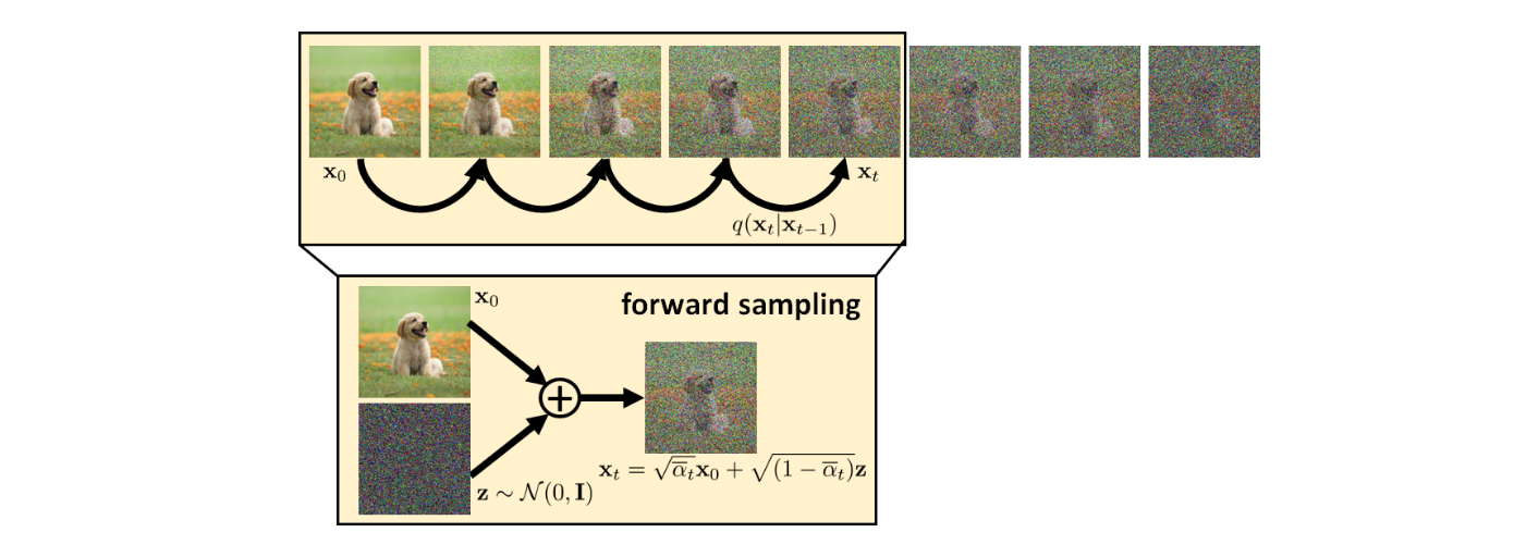In the ELBO we know

$${\mathbf{\mu }}_q({\mathbf{x}}_t,{\mathbf{x}}_0)=\frac{(1-{\overline{\alpha }}_{t-1})\sqrt{{\alpha }_t}}{1-{\overline{\alpha }}_t}{\mathbf{x}}_t+\frac{(1-{\alpha }_t)\sqrt{{\overline{\alpha }}_{t-1}}}{1-{\overline{\alpha }}_t}{\mathbf{x}}_0$$

But what about ${\mathbf{\mu }}_{\mathbf{\theta }}({\mathbf{x}}_t)$? Like in VAE's encoder, we could define it as

$$\underset{\text{A Network}}{\underbrace{{\mathbf{\mu }}_{\mathbf{\theta }}}}({\mathbf{x}}_t)\stackrel{\mathrm{def}}{=}\frac{(1-{\overline{\alpha }}_{t-1})\sqrt{{\alpha }_t}}{1-{\overline{\alpha }}_t}{\mathbf{x}}_t+\frac{(1-{\alpha }_t)\sqrt{{\overline{\alpha }}_{t-1}}}{1-{\overline{\alpha }}_t}\underset{\text{Another Network}}{\underbrace{{\hat{\mathbf{x}}}_{\mathbf{\theta }}({\mathbf{x}}_t)}}$$

where ${\hat{\mathbf{x}}}_{\mathbf{\theta }}$ is a trainable network with parameter $\mathbf{\theta }$. Now we get

$$\begin{array}{rl}\frac{1}{2{\sigma }_q^2(t)}\Vert {\mathbf{\mu }}_q({\mathbf{x}}_t,{\mathbf{x}}_0)-{\mathbf{\mu }}_{\mathbf{\theta }}({\mathbf{x}}_t){\Vert }^2& =\frac{1}{2{\sigma }_q^2(t)}{\Vert \frac{(1-{\alpha }_t)\sqrt{{\bar{\alpha }}_{t-1}}}{1-{\bar{\alpha }}_t}\left({\hat{\mathbf{x}}}_{\mathbf{\theta }}({\mathbf{x}}_t)-{\mathbf{x}}_0\right)\Vert }^2\\ & =\frac{1}{2{\sigma }_q^2(t)}\frac{(1-{\alpha }_t{)}^2{\bar{\alpha }}_{t-1}}{(1-{\bar{\alpha }}_t{)}^2}\Vert {\hat{\mathbf{x}}}_{\mathbf{\theta }}({\mathbf{x}}_t)-{\mathbf{x}}_0{\Vert }^2\end{array}$$

Therefore ELBO can be simplified into

$${\mathbb{E}}_{q_{\mathbf{\varphi }}({\mathbf{x}}_1|{\mathbf{x}}_0)}\left[\log p_{\mathbf{\theta }}({\mathbf{x}}_0|{\mathbf{x}}_1)\right]-\sum _{t=2}^T{\mathbb{E}}_{q_{\mathbf{\varphi }}({\mathbf{x}}_t|{\mathbf{x}}_0)}\left[\frac{1}{2{\sigma }_q^2(t)}\frac{(1-{\alpha }_t{)}^2{\bar{\alpha }}_{t-1}}{(1-{\bar{\alpha }}_t{)}^2}\Vert {\hat{\mathbf{x}}}_{\mathbf{\theta }}({\mathbf{x}}_t)-{\mathbf{x}}_0{\Vert }^2\right]$$

The first term is (using ${\alpha }_0=1$ and ${\alpha }_1={\bar{\alpha }}_1$)

$$\begin{array}{rl}\log p_{\mathbf{\theta }}({\mathbf{x}}_0|{\mathbf{x}}_1)& =\log \mathcal{N}({\mathbf{x}}_0\mid {\mathbf{\mu }}_{\mathbf{\theta }}({\mathbf{x}}_1),{\sigma }_q^2(1)\text{I})\propto -\frac{1}{2{\sigma }_q^2(q)}\Vert {\mathbf{\mu }}_{\mathbf{\theta }}({\mathbf{x}}_1)-{\mathbf{x}}_0{\Vert }^2\\ & =-\frac{1}{2{\sigma }_q^2(q)}{\Vert \frac{(1-{\overline{\alpha }}_0)\sqrt{{\alpha }_1}}{1-{\overline{\alpha }}_1}{\mathbf{x}}_1+\frac{(1-{\alpha }_1)\sqrt{{\overline{\alpha }}_0}}{1-{\overline{\alpha }}_1}{\hat{\mathbf{x}}}_{\mathbf{\theta }}({\mathbf{x}}_1)-{\mathbf{x}}_0\Vert }^2\\ & =-\frac{1}{2{\sigma }_q^2(q)}{\Vert \frac{(1-{\alpha }_1)}{1-{\overline{\alpha }}_1}{\hat{\mathbf{x}}}_{\mathbf{\theta }}({\mathbf{x}}_1)-{\mathbf{x}}_0\Vert }^2\\ & =-\frac{1}{2{\sigma }_q^2(q)}{\Vert {\hat{\mathbf{x}}}_{\mathbf{\theta }}({\mathbf{x}}_1)-{\mathbf{x}}_0\Vert }^2\end{array}$$

Now we get

$${\mathrm{ELBO}}_{\mathbf{\theta }}=-\sum _{t=1}^T{\mathbb{E}}_{q_{\mathbf{\varphi }}({\mathbf{x}}_t|{\mathbf{x}}_0)}\left[\frac{1}{2{\sigma }_q^2(t)}\frac{(1-{\alpha }_t{)}^2{\bar{\alpha }}_{t-1}}{(1-{\bar{\alpha }}_t{)}^2}\Vert {\hat{\mathbf{x}}}_{\mathbf{\theta }}({\mathbf{x}}_t)-{\mathbf{x}}_0{\Vert }^2\right]$$

And therefore the loss function

$$\boxed{{\mathbf{\theta }}^{\ast }=\underset{\mathbf{\theta }}{\mathrm{argmin}}\sum _{t=1}^T\frac{1}{2{\sigma }_q^2(t)}\frac{(1-{\alpha }_t{)}^2{\bar{\alpha }}_{t-1}}{(1-{\bar{\alpha }}_t{)}^2}{\mathbb{E}}_{q_{\mathbf{\varphi }}({\mathbf{x}}_t|{\mathbf{x}}_0)}\left[\Vert {\hat{\mathbf{x}}}_{\mathbf{\theta }}({\mathbf{x}}_t)-{\mathbf{x}}_0{\Vert }^2\right]}$$

Ignoring the constants and expectations, the main subject of interest, for a particular ${\mathbf{x}}_t$, is

$$\underset{\mathbf{\theta }}{\mathrm{argmin}}\Vert {\hat{\mathbf{x}}}_{\mathbf{\theta }}({\mathbf{x}}_t)-{\mathbf{x}}_0{\Vert }^2$$

So this is a denoising problem: we need to find a network ${\hat{\mathbf{x}}}_{\mathbf{\theta }}$ such that the denoised image ${\hat{\mathbf{x}}}_{\mathbf{\theta }}({\mathbf{x}}_t)$ will be close to the ground truth ${\mathbf{x}}_0$.

Training Process

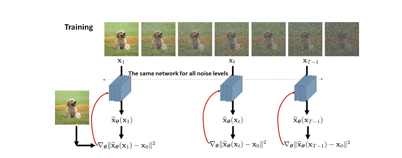For every image ${\mathbf{x}}_0$ in the training dataset:

• Repeat the following steps until convergence
• Pick a random time stamp $t\sim \mathrm{Uniform}[1,T]$
• Draw a sample ${\mathbf{x}}_t\sim q_{\mathbf{\varphi }}({\mathbf{x}}_t|{\mathbf{x}}_0)=\mathcal{N}({\mathbf{x}}_t\mid \sqrt{{\bar{\alpha }}_t}{\mathbf{x}}_0,(1-{\bar{\alpha }}_t)\text{I})$, i.e.,

$${\mathbf{x}}_t={\bar{\alpha }}_t{\mathbf{x}}_0+\sqrt{(1-{\bar{\alpha }}_t)}\mathbf{z},\mathbf{z}\sim \mathcal{N}(0,\text{I})$$

• Take gradient descent step on

$${\nabla }_{\mathbf{\theta }}\Vert {\hat{\mathbf{x}}}_{\mathbf{\theta }}({\mathbf{x}}_t)-{\mathbf{x}}_0{\Vert }^2$$

Inference Process

Once the denoiser ${\hat{\mathbf{x}}}_{\mathbf{\theta }}$ is trained, we can apply it to do the inference. The inference is about sampling images from the distributions $p_{\mathbf{\theta }}({\mathbf{x}}_{t-1}|{\mathbf{x}}_t)$ over the sequence of states ${\mathbf{x}}_T,{\mathbf{x}}_{T-1},\dots ,{\mathbf{x}}_1$. Since it is the reverse diffusion process, we need to do it recursively via:

$$\begin{array}{rl}{\mathbf{x}}_{t-1}\sim p_{\mathbf{\theta }}({\mathbf{x}}_{t-1}|{\mathbf{x}}_t)& =\mathcal{N}({\mathbf{x}}_{t-1}\mid {\mathbf{\mu }}_{\mathbf{\theta }}({\mathbf{x}}_t),{\sigma }_q^2(t)\text{I})\\ & ={\mathbf{\mu }}_{\mathbf{\theta }}({\mathbf{x}}_t)+{\sigma }_q^2(t)\mathbf{z},\mathbf{z}\sim \mathcal{N}(0,\text{I})\\ & =\frac{(1-{\overline{\alpha }}_{t-1})\sqrt{{\alpha }_t}}{1-{\overline{\alpha }}_t}{\mathbf{x}}_t+\frac{(1-{\alpha }_t)\sqrt{{\overline{\alpha }}_{t-1}}}{1-{\overline{\alpha }}_t}{\hat{\mathbf{x}}}_{\mathbf{\theta }}({\mathbf{x}}_t)+{\sigma }_q(t)\mathbf{z}\end{array}$$

This leads to the inferencing algorithm

• Given a white noise vector ${\mathbf{x}}_T\sim \mathcal{N}(0,\text{I})$
• Repeat the following for $t=T,T-1,\dots ,1$
  • Calculate ${\hat{\mathbf{x}}}_{\mathbf{\theta }}({\mathbf{x}}_t)$ using the trained denoiser
  • Update according to

$${\mathbf{x}}_{t-1}=\frac{(1-{\overline{\alpha }}_{t-1})\sqrt{{\alpha }_t}}{1-{\overline{\alpha }}_t}{\mathbf{x}}_t+\frac{(1-{\alpha }_t)\sqrt{{\overline{\alpha }}_{t-1}}}{1-{\overline{\alpha }}_t}{\hat{\mathbf{x}}}_{\mathbf{\theta }}({\mathbf{x}}_t)+{\sigma }_q(t)\mathbf{z},\mathbf{z}\sim \mathcal{N}(0,\text{I})$$

Inversion by Direct Denoising (InDI)

If we look at the updating equation above, we could see the following form:

$${\mathbf{x}}_{t-1}=\left(\text{something}\right)\cdot {\mathbf{x}}_t+\left(\text{something else}\right)\cdot \text{denoise}({\mathbf{x}}_t)+\text{noise}$$

The first term is easy to understand, but what is "denoise"?

More about Denoise

Denoising is a generic procedure that removes noise from a noisy image. Given the observation model

$$\mathbf{y}=\mathbf{x}+\mathbf{ϵ},\mathbf{ϵ}\sim \mathcal{N}(0,\text{I})$$

A classical solution to find an estimator $g(\cdot )$ such that the mean squared error is minimized is

$$\begin{array}{rl}\mathrm{denoise}(\mathbf{y})& =\underset{g}{\mathrm{argmin}}{\mathbb{E}}_{\mathbf{x},\mathbf{y}}\left[\Vert g(\mathbf{y})-\mathbf{x}{\Vert }^2\right]\\ & =\text{some steps}\\ & =\mathbb{E}[\mathbf{x}|\mathbf{y}]\end{array}$$

So, if we assume that during the forward path

$${\mathbf{x}}_t={\mathbf{x}}_{t-1}+{\mathbf{ϵ}}_{t-1},\mathbf{ϵ}\sim \mathcal{N}(0,\text{I})$$

we can find the solution of denoiser

$$\mathrm{denoise}({\mathbf{x}}_t)=\mathbb{E}\left[{\mathbf{x}}_{t-1}|{\mathbf{x}}_t\right]$$

Such a denoiser is called the minimum mean squared error (MMSE) denoiser. MMSE denoiser is not the "best" denoiser; It is only the optimal denoiser with respect to the mean squared error. Since mean squared error is never a good metric for image quality, minimizing the MSE will not necessarily give us a better image.

Incremental Denoising Steps

The previous section tells us that an MMSE denoiser is equivalent to the conditional expectation of the posterior distribution. Now we introduce incremental denoising. Suppose that we have a clean image ${\mathbf{x}}_0$ and a noise image $\mathbf{y}$. Our goal is to form a linear combination of ${\mathbf{x}}_0$ and $\mathbf{y}$ via a simple equation

$${\mathbf{x}}_t=(1-t){\mathbf{x}}_0+t\mathbf{y},0\le t\le 1$$

Now, consider a small step $\tau :0\le \tau <t\le 1$, then it holds that

$$\mathbb{E}[{\mathbf{x}}_{t-\tau }|{\mathbf{x}}_t]=\left(1-\frac{\tau }{t}\right)\underset{\text{current estimate}}{\underbrace{{\mathbf{x}}_t}}+\frac{\tau }{t}\underset{\text{denoised}}{\underbrace{\mathbb{E}[{\mathbf{x}}_0|{\mathbf{x}}_t]}}$$

If we define ${\hat{\mathbf{x}}}_{t-\tau }$ as the left hand side, replace ${\mathbf{x}}_t$ by ${\hat{\mathbf{x}}}_t$, and write $\mathbb{E}[{\mathbf{x}}_0|{\mathbf{x}}_t]$ as $\mathrm{denoise}({\hat{\mathbf{x}}}_t)$, then the above equation will become

$${\hat{\mathbf{x}}}_{t-\tau }=\left(1-\frac{\tau }{t}\right)\cdot {\hat{\mathbf{x}}}_t+\frac{\tau }{t}\mathrm{denoise}({\hat{\mathbf{x}}}_t)$$

where $\tau$ is a small step in time. This equation gives us an inference step. If you tell us the denoiser and suppose that you start with a noisy image $\mathbf{y}$, then you can iteratively apply this equation to retrieve the images ${\hat{\mathbf{x}}}_{t-1},{\hat{\mathbf{x}}}_{t-2},\dots ,{\hat{\mathbf{x}}}_0$

Equivalent Interpretations

Predicting noises

As discussed above, a Variational Diffusion Model can be trained by simply learning a neural network to predict the original natural image ${\mathbf{x}}_0$ form an arbitrary noised version ${\mathbf{x}}_t$ and its time index $t$.

This interpretation is from the parameterization of ${\mathbf{x}}_t$, that is

$${\mathbf{x}}_t=\sqrt{{\bar{\alpha }}_t}{\mathbf{x}}_0+\sqrt{(1-{\bar{\alpha }}_t)}\mathbf{z},\mathbf{z}\sim \mathcal{N}(0,\text{I})$$

And we can rewrite this to

$${\mathbf{x}}_0=\frac{{\mathbf{x}}_t-\sqrt{1-{\bar{\alpha }}_t}\mathbf{z}}{\sqrt{{\bar{\alpha }}_t}}$$

Now we can change ${\mathbf{\mu }}_q({\mathbf{x}}_t,{\mathbf{x}}_0)$ to a function of ${\mathbf{x}}_t,\mathbf{z}$ rather than ${\mathbf{x}}_0,\mathbf{z}$, that is

$$\begin{array}{rl}{\mathbf{\mu }}_q({\mathbf{x}}_t,{\mathbf{x}}_0)& =\frac{\sqrt{{\alpha }_t}(1-{\bar{\alpha }}_{t-1}){\mathbf{x}}_t+\sqrt{{\bar{\alpha }}_{t-1}}(1-{\alpha }_t){\mathbf{x}}_0}{1-{\bar{\alpha }}_t}\\ & =\frac{\sqrt{{\alpha }_t}(1-{\bar{\alpha }}_{t-1}){\mathbf{x}}_t+\sqrt{{\bar{\alpha }}_{t-1}}(1-{\alpha }_t)\frac{{\mathbf{x}}_t-\sqrt{1-{\bar{\alpha }}_t}\mathbf{z}}{\sqrt{{\bar{\alpha }}_t}}}{1-{\bar{\alpha }}_t}\\ & =\frac{\sqrt{{\alpha }_t}(1-{\bar{\alpha }}_{t-1}){\mathbf{x}}_t}{1-{\bar{\alpha }}_t}+\frac{(1-{\alpha }_t){\mathbf{x}}_t}{(1-{\bar{\alpha }}_t)\sqrt{{\alpha }_t}}-\frac{(1-{\alpha }_t)\sqrt{1-{\bar{\alpha }}_t}\mathbf{z}}{(1-{\bar{\alpha }}_t)\sqrt{{\alpha }_t}}\\ & =\left(\frac{{\alpha }_t(1-{\bar{\alpha }}_{t-1})}{(1-{\bar{\alpha }}_t)\sqrt{{\alpha }_t}}+\frac{1-{\alpha }_t}{(1-{\bar{\alpha }}_t)\sqrt{{\alpha }_t}}\right){\mathbf{x}}_t-\frac{1-{\alpha }_t}{\sqrt{1-{\bar{\alpha }}_t}\sqrt{{\alpha }_t}}\mathbf{z}\\ & =\frac{{\alpha }_t-{\bar{\alpha }}_t+1-{\alpha }_t}{(1-{\bar{\alpha }}_t)\sqrt{{\alpha }_t}}{\mathbf{x}}_t-\frac{1-{\alpha }_t}{\sqrt{1-{\bar{\alpha }}_t}\sqrt{{\alpha }_t}}\mathbf{z}\\ & =\frac{1}{\sqrt{{\alpha }_t}}{\mathbf{x}}_t-\frac{1-{\alpha }_t}{\sqrt{1-{\bar{\alpha }}_t}\sqrt{{\alpha }_t}}\mathbf{z}\end{array}$$

Therefore, now we could set our predicted transition mean as

$${\mathbf{\mu }}_{\mathbf{\theta }}({\mathbf{x}}_t,t)=\frac{1}{\sqrt{{\alpha }_t}}{\mathbf{x}}_t-\frac{1-{\alpha }_t}{\sqrt{1-{\bar{\alpha }}_t}\sqrt{{\alpha }_t}}{\hat{\mathbf{z}}}_{\mathbf{\theta }}({\mathbf{x}}_t,t)$$

And after some calculations, we just need to optimize

$$\boxed{{\mathbf{\theta }}^{\ast }=\underset{\mathbf{\theta }}{\mathrm{argmin}}\sum _{t=1}^T\frac{1}{2{\sigma }_q^2(t)}\frac{(1-{\alpha }_t{)}^2}{(1-{\bar{\alpha }}_t{)}^2{\alpha }_t}{\mathbb{E}}_{q_{\mathbf{\varphi }}({\mathbf{x}}_t|{\mathbf{x}}_0)}\left[\Vert {\hat{\mathbf{z}}}_{\mathbf{\theta }}({\mathbf{x}}_t)-{\mathbf{z}}_0{\Vert }^2\right]}$$

We have therefore shown that learning a VDM by predicting the original image ${\mathbf{x}}_0$ is equivalent to learning to predict the noise; empirically, however, some works have found that predicting the noise resulted in better performance

Predicting scores

As we have concluded

$$q({\mathbf{x}}_t|{\mathbf{x}}_0)=\mathcal{N}({\mathbf{x}}_t\mid \sqrt{{\bar{\alpha }}_t}{\mathbf{x}}_0,(1-{\bar{\alpha }}_t)\text{I})$$

by Tweedie's Formula, we have

$$\mathbb{E}[{\mathbf{\mu }}_{{\mathbf{x}}_t}|{\mathbf{x}}_t]={\mathbf{x}}_t+(1-{\bar{\alpha }}_t){\nabla }_{{\mathbf{x}}_t}\log p({\mathbf{x}}_t)$$

And we know the best estimate for the true mean of ${\mathbf{x}}_t$ given ${\mathbf{x}}_0$ is $\sqrt{{\bar{\alpha }}_t}{\mathbf{x}}_0$, now we get (write ${\nabla }_{{\mathbf{x}}_t}$ as $\nabla$ for convenience)

$$\sqrt{{\bar{\alpha }}_t}{\mathbf{x}}_0={\mathbf{x}}_t+(1-{\bar{\alpha }}_t)\nabla \log p({\mathbf{x}}_t)$$

Now we get another way to express ${\mathbf{\mu }}_q({\mathbf{x}}_t,{\mathbf{x}}_0)$

$$\begin{array}{rl}{\mathbf{\mu }}_q({\mathbf{x}}_t,{\mathbf{x}}_0)& =\frac{\sqrt{{\alpha }_t}(1-{\bar{\alpha }}_{t-1}){\mathbf{x}}_t+\sqrt{{\bar{\alpha }}_{t-1}}(1-{\alpha }_t){\mathbf{x}}_0}{1-{\bar{\alpha }}_t}\\ & =\frac{\sqrt{{\alpha }_t}(1-{\bar{\alpha }}_{t-1}){\mathbf{x}}_t+\sqrt{{\bar{\alpha }}_{t-1}}(1-{\alpha }_t)\frac{{\mathbf{x}}_t+(1-{\bar{\alpha }}_t)\nabla \log p({\mathbf{x}}_t)}{\sqrt{{\bar{\alpha }}_t}}}{1-{\bar{\alpha }}_t}\\ & =\frac{\sqrt{{\alpha }_t}(1-{\bar{\alpha }}_{t-1}){\mathbf{x}}_t}{1-{\bar{\alpha }}_t}+\frac{(1-{\alpha }_t){\mathbf{x}}_t}{(1-{\bar{\alpha }}_t)\sqrt{{\alpha }_t}}+\frac{(1-{\alpha }_t)(1-{\bar{\alpha }}_t)\nabla \log p({\mathbf{x}}_t)}{(1-{\bar{\alpha }}_t)\sqrt{{\alpha }_t}}\\ & =\left(\frac{{\alpha }_t(1-{\bar{\alpha }}_{t-1})}{(1-{\bar{\alpha }}_t)\sqrt{{\alpha }_t}}+\frac{1-{\alpha }_t}{(1-{\bar{\alpha }}_t)\sqrt{{\alpha }_t}}\right){\mathbf{x}}_t+\frac{1-{\alpha }_t}{\sqrt{{\alpha }_t}}\nabla \log p({\mathbf{x}}_t)\\ & =\frac{{\alpha }_t-{\bar{\alpha }}_t+1-{\alpha }_t}{(1-{\bar{\alpha }}_t)\sqrt{{\alpha }_t}}{\mathbf{x}}_t+\frac{1-{\alpha }_t}{\sqrt{{\alpha }_t}}\nabla \log p({\mathbf{x}}_t)\\ & =\frac{1}{\sqrt{{\alpha }_t}}{\mathbf{x}}_t+\frac{1-{\alpha }_t}{\sqrt{{\alpha }_t}}\nabla \log p({\mathbf{x}}_t)\end{array}$$

Therefore, we can also set our approximate denoising transition mean ${\mathbf{\mu }}_{\mathbf{\theta }}({\mathbf{x}}_t)$ as

$${\mathbf{\mu }}_{\mathbf{\theta }}({\mathbf{x}}_t)=\frac{1}{\sqrt{{\alpha }_t}}{\mathbf{x}}_t+\frac{1-{\alpha }_t}{\sqrt{{\alpha }_t}}{\mathbf{s}}_{\mathbf{\theta }}({\mathbf{x}}_t,t)$$

And the corresponding optimization problem becomes

$$\boxed{{\mathbf{\theta }}^{\ast }=\underset{\mathbf{\theta }}{\mathrm{argmin}}\sum _{t=1}^T\frac{1}{2{\sigma }_q^2(t)}\frac{(1-{\alpha }_t{)}^2}{{\alpha }_t}{\mathbb{E}}_{q_{\mathbf{\varphi }}({\mathbf{x}}_t|{\mathbf{x}}_0)}\left[\Vert {\mathbf{s}}_{\mathbf{\theta }}({\mathbf{x}}_t)-\nabla \log p({\mathbf{x}}_t){\Vert }^2\right]}$$

One more problem is how to calculate $\nabla \log p({\mathbf{x}}_t)$, this would be easy if we apply the relationship used in predicting noises

$${\mathbf{x}}_0=\frac{{\mathbf{x}}_t-\sqrt{1-{\bar{\alpha }}_t}\mathbf{z}}{\sqrt{{\bar{\alpha }}_t}}$$

This is equal to

$${\mathbf{x}}_0=\frac{{\mathbf{x}}_t+(1-{\bar{\alpha }}_t)\nabla \log p({\mathbf{x}}_t)}{\sqrt{{\bar{\alpha }}_t}}$$

Now we get

$$\nabla \log p({\mathbf{x}}_t)=-\frac{1}{\sqrt{1-{\bar{\alpha }}_t}}\mathbf{z}$$

Tip

The score function measures how to move in data space to maximize the log probability; intuitively, since the source noise is added to a natural image to corrupt it, moving in its opposite direction "denoises" the image and would be the best update to increase the subsequent log probability.

Score-Matching Langevin Dynamics (SMLD)

In this section we dive into the intuition of the score-matching interpretation.

Energy-based Models

To begin to understand why optimizing a score function makes sense, we shall first introduce energy-based models. Remember the form of Boltzmann Distribution, we have

$$p_{\mathbf{\theta }}(\mathbf{x})=\frac{1}{Z_{\mathbf{\theta }}}\exp \left[-f_{\mathbf{\theta }}(\mathbf{x})\right]$$

where $f_{\mathbf{\theta }}$ is an arbitrarily flexible, parameterizable function called the energy function, and $Z_{\mathbf{\theta }}$ is a normalizing constant to ensure that $\int p_{\mathbf{\theta }}(\mathbf{x})\mathrm{d}x=1$. One way to learn this distribution is MLE, but this requires tractably computing the normalizing constant $Z_{\mathbf{\theta }}=\int \exp \left[-f_{\mathbf{\theta }}(\mathbf{x})\right]$, which may not be possible for complex $f_{\mathbf{\theta }}(\mathbf{x})$ functions.

One way to avoid calculating or modeling the normalization constant is by using a neural network ${\mathbf{s}}_{\mathbf{\theta }}(\mathbf{x})$ to learn the score function $\nabla \log p(\mathbf{x})$ of distribution $p(\mathbf{x})$ instead. This can be done by taking the derivative of the log of both sides of the equation above

$$\begin{array}{rl}{\nabla }_{\mathbf{x}}\log p_{\mathbf{\theta }}(\mathbf{x})& ={\nabla }_{\mathbf{x}}\log \left\{\frac{1}{Z_{\mathbf{\theta }}}\exp \left[-f_{\mathbf{\theta }}(\mathbf{x})\right]\right\}\\ & ={\nabla }_{\mathbf{x}}\log \frac{1}{Z_{\mathbf{\theta }}}+{\nabla }_{\mathbf{x}}\log \exp \left[-f_{\mathbf{\theta }}(\mathbf{x})\right]\\ & =-{\nabla }_{\mathbf{x}}{f}_{\mathbf{\theta }}(\mathbf{x})\\ & \approx {\mathbf{s}}_{\mathbf{\theta }}(\mathbf{x})\end{array}$$

which can be freely represented as a neural network without involving any normalization constants. The score model can be optimized by minimizing the Fisher Divergence with the ground truth score function

$${\mathbb{E}}_{p(\mathbf{x})}\left[\Vert {\mathbf{s}}_{\mathbf{\theta }}(\mathbf{x})-\nabla \log p(\mathbf{x}){\Vert }^2\right]$$

Langevin Dynamics

Imagine that we are given a distribution $p(\mathbf{x})$ and suppose that we want to draw samples from $p(\mathbf{x})$. Langevin dynamics is an iterative procedure that allows us to draw samples according to the following equation

$${\mathbf{x}}_{t+1}={\mathbf{x}}_t+\tau {\nabla }_{\mathbf{x}}\log p({\mathbf{x}}_t)+\sqrt{2\tau }\mathbf{z},\mathbf{z}\sim \mathcal{N}(0,\text{I})$$

where $\tau$ is the step size which users can control, and ${\mathbf{x}}_0$ is white noise.

Note that if we ignore the noise term $\sqrt{2\tau }\mathbf{z}$ at the end, the Langevin dynamics equation is literally gradient descent. The descent ${\nabla }_{\mathbf{x}}\log p(\mathbf{x})$ is carefully chosen that ${\mathbf{x}}_t$ will converge to the distribution $p(\mathbf{x})$.

The goal of this descent sampling process is to find a $\mathbf{x}$ where the probability is the highest, which is equivalent to solving the optimization

$${\mathbf{x}}^{\ast }=\underset{\mathbf{x}}{\mathrm{argmax}}\log p(\mathbf{x})$$

Warning

Note that this is not MLE. In maximum likelihood, the data point $\mathbf{x}$ is fixed but the model parameters are changing. Here, the model parameters are fixed but the data point is changing.

And now we can understand the noise term $\sqrt{2\tau }\mathbf{z}$, which literally changes the gradient descent to stochastic gradient descent. Instead of shooting for the deterministic optimum, the stochastic gradient descent climbs up the hill randomly, so that there would be a lower probability to stuck into a local maximum

However, we actually do not care about the maximum of $p(\mathbf{x})$, which is the final goal of the descent process. Instead, we care about the sampling process itself. As well as our descent algorithm is good at find peaks, then by repeatedly initialize the algorithm at a uniformly distributed location, we will eventually collects samples that will follow the distribution we want to match.

Info

Suppose we initialize $10000$ uniformly distributed samples $x_0\sim \mathrm{Uniform}[-3,3]$. We run Langevin updates for $t=100$ steps. The histograms of generated samples are shown in the figures below

In summary, Langevin dynamics gives us a more intuitive vision into the score-matching problem in energy-based models. In energy-based models, we learn the distribution of $p_{\mathbf{\theta }}$ by matching a score function ${\mathbf{s}}_{\mathbf{\theta }}$ with $\nabla \log p(\mathbf{x})$. On the other hand, if we find a good estimation ${\mathbf{s}}_{\mathbf{\theta }}$ of the descent term $\nabla \log p(\mathbf{x})$ in Langevin dynamics, the sampling process would do better in finding a peak in the neighborhood of its initial state ${\mathbf{x}}_0$, so that by initialize the ${\mathbf{x}}_0$ uniformly in the interval we interested with, the sampling would follow the $p(\mathbf{x})$ we want to approximate.